Improving multisite precipitation generators based on generalised linear models

Precipitation generators are statistical models used to produce synthetic sequences of (multisite) precipitation for hydrological applications such as flood risk assessment and water resource management. Among these, approaches based on generalized linear models (GLMs) are widely used and often perform competitively with state-of-the-art alternatives, but they face limitations in representing seasonal variation in extremes and in flexibly capturing covariate effects on the precipitation distribution. In this paper, we extend the GLM framework in two directions. First, we introduce generalised additive models for location, scale and shape (GAMLSS) for precipitation generation. These models allow the use of spline-based model terms to flexibly capture covariate effects and allow covariates to influence multiple distributional parameters, thereby increasing flexibility in representing variation in both the mean and variance of the precipitation distribution. Second, we adapt a transformed Gaussian fields approach to jointly account for spatial dependence in both precipitation occurrence and intensity, thus allowing for potential cross-dependence between the two. A further contribution is to investigate the sensitivity of model performance to data resolution, highlighting that rounding in data pre-processing can substantially affect the reproduction of extremes. Using a well-studied daily precipitation dataset, we demonstrate that these extensions improve the realism of simulated sequences, particularly with respect to extremes, and capture spatial dependence well in both occurrence and intensity.

1 Introduction

Precipitation is a key driver of most hydrological systems, so that the representation of precipitation variability in both space and time is often critical when studying the behaviour of such systems – for example in flood risk assessment or water resource management. To characterise this variability and its effect, a common approach is to use stochastic or statistical models to generate synthetic sequences of precipitation and other relevant quantities, and to use the resulting sequences as inputs to hydrological models; see Beven (2021), for example.

The development of techniques for producing sequences of precipitation and other variables, preserving relationships between them, can be traced back to the “weather generator” of Richardson (1981). This built on a large body of literature focused on the development of stochastic and statistical models specifically for precipitation without considering other variables: such models are referred to henceforth as “precipitation generators”. Some reviews, from differing perspectives, are given by Maraun et al. (2010); Chandler et al. (2014); and Northrop (2024).

In the original weather generator of Richardson (1981), daily precipitation occurrence is modelled as a Markov chain with wet-day precipitation intensities generated independently using either exponential or gamma distributions. The approach has several known deficiencies, including difficulty in reproducing the distributions of extreme precipitation and of wet and dry spell durations. Several alternative approaches have been proposed, some designed explicitly to overcome these deficiencies. For example, the LARS-WG generator of Semenov et al. (1998) models spell length distributions directly, while Furrer and Katz (2008) use heavy-tailed distributions for wet-day intensity to improve the representation of extremes. Other approaches include those based on resampling the historical record (Buishand and Brandsma, 2001; Beersma and Buishand, 2003), those based on transformed Gaussian distributions (Stehlík and Bárdossy, 2002); and those based on Hidden Markov Models (HMMs) in which different precipitation distributions are associated with each of a collection of underlying “weather states” (Charles et al., 1999; Ailliot et al., 2009; Holsclaw et al., 2016; Dawkins et al., 2022).

Many studies have been carried out to compare subsets of these approaches, by evaluating their ability to reproduce key features of observed weather sequences using frameworks such as that of Maraun et al. (2015). The results from some of these studies should be treated with caution, however, because the effective use of some methods requires a high degree of technical awareness: in the hands of a trained user, such methods are therefore likely to outperform the “off-the-shelf” implementations that are sometimes used in comparison studies. Our own experience is that when implemented with insight and understanding, several of the more sophisticated modelling approaches are capable of reproducing a wide range of properties of observed precipitation sequences over a range of spatial scales, including basic summary statistics, measures of temporal persistence and extremal behaviour.

One of these “more sophisticated” approaches is based on generalised linear models (GLMs) which, notwithstanding the caveats above regarding comparison studies, are often found to perform well in absolute terms and to compete favourably with other state-of-the-art approaches such as HMMs (e.g. Frost et al., 2011; Kenabatho et al., 2012; Mockler et al., 2016; Asong et al., 2016; Ayar et al., 2016; Chun et al., 2017; Tosonoğlu and Onof, 2017). Indeed, some other approaches can be regarded as special cases of GLMs (e.g. Grunwald and Jones, 2000). As well as the potential to produce sequences with realistic spatial, temporal and inter-variable dependence structures over a range of scales, the GLM-based approach is able to represent systematic variation over space and time, including under scenarios of climate change (see Sect. 2.2); to generate sequences at locations for which no data are available; and to cope with missing values and unequal record lengths in the historical records used for model calibration (Chandler, 2020).

Despite the strengths of the GLM-based approach to precipitation generation, it has some known deficiencies. For example, it typically struggles to capture seasonal variation in extreme precipitation – a phenomenon first noted by Yang et al. (2005b). Other precipitation generators suffer from similar problems: indeed, to address the issue in applications for which the reproduction of extremes is critical, some authors have advocated the use of models in which precipitation intensities are considered to be drawn from distributions with two separate parts, one for the main body of the data and the other for the extremes (e.g. Cameron et al., 2001; Furrer and Katz, 2008). Arguably, however, this addresses the symptom of the problem rather than its cause, which, for GLMs at least, is likely to be partly a lack of flexibility in representing variation in different aspects of the precipitation distribution. This is because, in standard applications of the GLM methodology to daily precipitation, non-zero precipitation intensities are modelled using gamma distributions in which the standard deviation is proportional to the mean as discussed in Sect. 3.1 below. This restriction is made for mathematical and computational convenience, but it lacks physical justification: it is therefore worth investigating whether the reproduction of extremal behaviour can be improved by relaxing it.

Another feature of GLMs is that the means of the daily precipitation distributions are related to linear combinations of predictors (referred to as “covariates” below), representing systematic variation associated with seasonality, regional variation, large-scale atmospheric conditions, previous days' weather, and so forth: again, Sect. 3.1 provides details. A further potential enhancement is to relax the requirement for the covariates to be combined linearly and, instead, to let the data determine the most appropriate form of the relationship. Generalised Additive Models (GAMs) allow this, via smooth semiparametric representations of the covariate effects on the means of the daily precipitation distributions. GAMs have been developed for daily precipitation series by, for example, Hyndman and Grunwald (2000); Beckmann and Buishand (2002) and Underwood (2008) – although, again, they impose a fixed relationship between the mean and standard deviation of the intensity distribution.

Against this background, the primary contribution of the present paper is to examine the effect of allowing a more flexible modelling framework in which covariates are allowed to influence multiple aspects of the daily precipitation distribution, both parametrically and semi-parametrically. Our working hypothesis is that the known deficiencies of GLM-based generators – in particular their tendency to misrepresent seasonal precipitation extremes – reflect primarily a lack of flexibility in representing variation in the scale of the intensity distribution and in the functional form of covariate effects, rather than a fundamental misspecification of the distributional family itself; we therefore retain the widely-used gamma distribution for precipitation intensities throughout. To test this hypothesis, we use the class of Generalised Additive Models for Location, Scale and Shape (GAMLSS; Rigby and Stasinopoulos, 2005) which, in principle, allow both parametric and semiparametric representation of covariate effects on the first four moments of precipitation intensity. GAMLSS do not appear to have been used previously as precipitation generators, although they have been used in related areas such as the linking of local precipitation climatologies to large-scale atmospheric conditions (e.g. Villarini et al., 2010; Rashid et al., 2016); the analysis of trends in extreme precipitation (e.g. Gu et al., 2019; Liu et al., 2022); and the characterisation of nonstationarity in the frequency and severity of floods and droughts (e.g. Villarini et al., 2009; López and Francés, 2013; Machado et al., 2015; Wang et al., 2015; Rashid and Beecham, 2019).

While evaluating the performance of the GLM- and GAMLSS-based approaches in the case study described in Sect. 2, the reproduction of extreme precipitation was found to be surprisingly sensitive to the recording resolution of the data. For example, the results can change appreciably if the data are rounded to the nearest 0.5 mm prior to analysis, as is sometimes done to reduce the effect of inconsistent recording practices over time or between stations (e.g. Ambrosino et al., 2014). Although it is known that modelling results can be sensitive to the way in which small precipitation values are recorded (Yang et al., 2006), this more general effect of rounding is, to our knowledge, not widely appreciated. A secondary contribution of the paper is to examine this effect, therefore.

GLM-based precipitation generators treat precipitation occurrence and intensity separately (see Sect. 3.1). This is unrestrictive when considering a single location, because the cumulative distribution function of the precipitation amount (Y, say) can always be written as

$$\begin{array}{rl}{F}_Y\left(y\right):=P(Y\le y)=& P(Y\le y|Y=\mathrm{0}\left)P\right(Y=\mathrm{0})\\ & +P(Y\le y|Y>\mathrm{0}\left)P\right(Y>\mathrm{0})\end{array}$$

where the notation P(A|B) denotes the conditional probability of an event A given that B has occurred. The expression $P(Y>\mathrm{0})=\mathrm{1}-P(Y=\mathrm{0})$ is the probability of precipitation occurrence; while the conditional probability $P(Y<y|Y>\mathrm{0})$ can be deduced from a model for non-zero precipitation intensity and, trivially, $P(Y\le y|Y=\mathrm{0})=\mathrm{1}$ for all y≥0.

When considering daily precipitation at multiple locations, however, it is necessary to consider the dependence between different sites on the same day. To model this dependence, intensities are again treated separately from occurrence in most GLM-based precipitation generators. When using the resulting models to generate synthetic multisite precipitation sequences therefore, the “dry” sites are ignored when generating non-zero intensities at “wet” sites so that the methodology is not capable of (for example) systematically producing lower intensities at locations close to dry sites. The extent to which this is a problem is probably application-specific, but it is avoided in some other approaches, such as those building on the work of Bárdossy and Plate (1992), which uses transformations of Gaussian random fields. A final contribution of the present paper is thus to adapt the transformed Gaussian fields approach to the context of GLMs and GAMLSS, so as to represent inter-site dependence in precipitation and occurrence simultaneously.

The extensions of the basic GLM methodology are demonstrated using a dataset similar to that used by Yang et al. (2005b): this allows for a straightforward evaluation of their effects in a setting where the performance of GLMs is well understood. The dataset is described in the next section, after which Sect. 3 provides a brief review of GLM-based precipitation generators and describes the proposed extensions. The performance of the methods is assessed and compared in Sect. 4; Sect. 5 concludes.

2 Study area and data

The study area considered in Yang et al. (2005b) has dimensions around 50 km × 40 km and is centred on the catchment of the river Blackwater, a subtributary of the Thames in southern England. As illustrated in Fig. 1, the region has modest topographical variation: altitudes range from near sea-level in the Thames floodplain in the north-east to almost 300 m at the highest points of two escarpments running roughly East-West. The region has a humid temperate oceanic climate (Beck et al., 2018), with a mean annual precipitation of around 750 mm and precipitation occurring throughout the year. Much of the precipitation is associated with large-scale synoptic systems transporting moisture from the Atlantic, although precipitation extremes in summer are often associated with more localised convective events (Mayes, 2013).

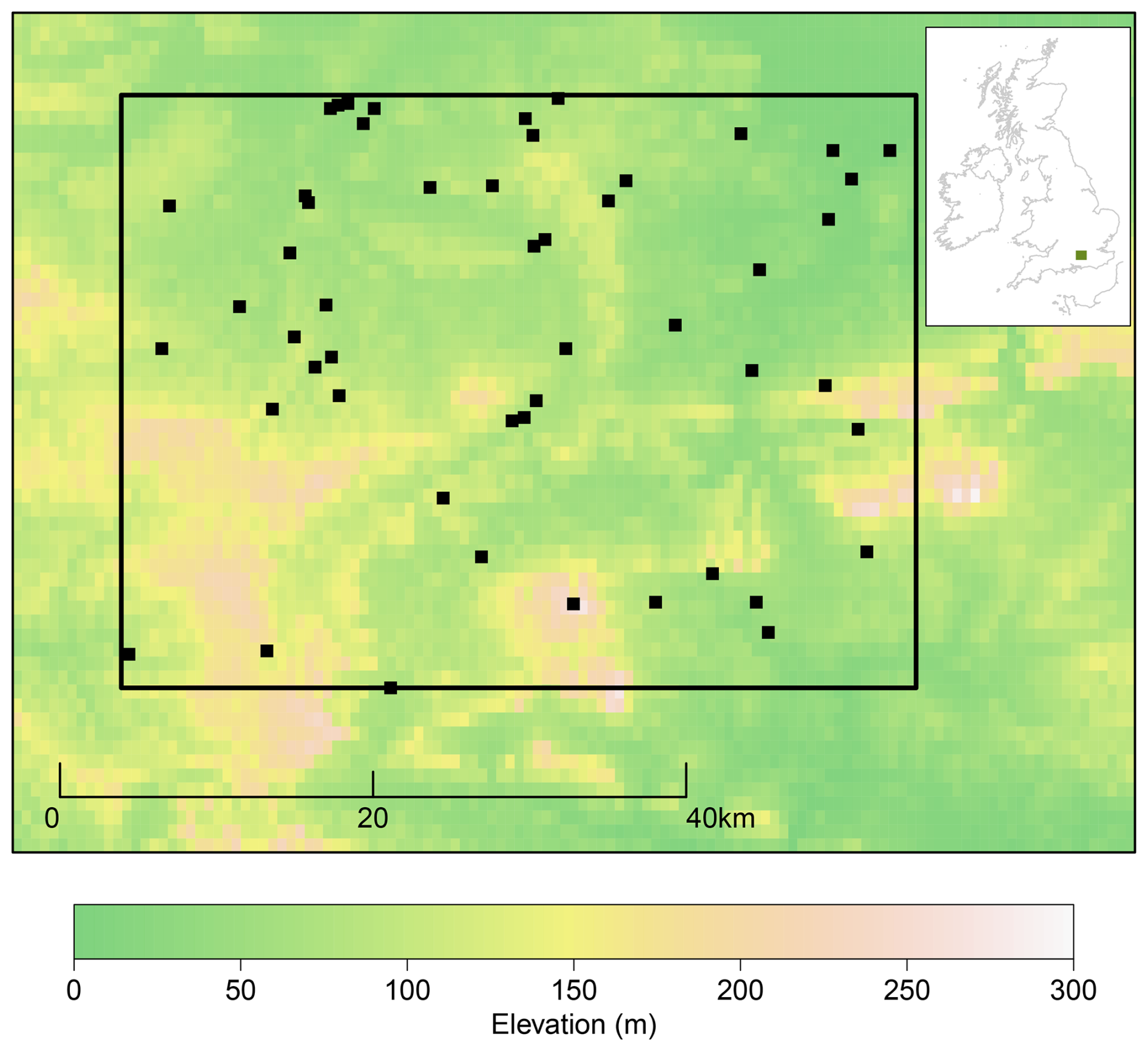
Figure 1 Topographical map of the study area (solid rectangle), with locations of the 51 gauges providing data used in the study. The inset shows the location of the study area within the British Isles.

2.1 Precipitation data

The present study uses a more extensive daily precipitation dataset than that considered by Yang et al. (2005b), from a network of 51 stations at locations shown in Fig. 1. These data are a subset of the MIDAS precipitation dataset (Met Office, 2006). Records cover the period from 1923 to 2022, although few stations were operational during the first few decades of this period. Moreover, data on atmospheric covariates (see below) are only available from 1959 onwards: we therefore restrict attention to the period 1959–2022. The complete MIDAS precipitation dataset includes data from 171 stations that were operational at some time during this period; the 51 selected stations were identified based on extensive quality checks. Specifically, records were retained only if they were nominally operational for at least 10 years and had fewer than 10 % of values missing. Furthermore, since operational difficulties and data quality problems during a given period can often lead to anomalies in the recorded proportions of wet days at a site (e.g. Chandler et al., 2011), such anomalies were identified from the residuals of a two-way Analysis of Variance (ANOVA) fitted to the annual proportions of wet days at each location. Periods of dubious data quality identified from this exercise were also excluded from the subsequent analysis, as were several values that were (i) unusually large (ii) recorded on the last day of a calendar month and (iii) the only value recorded at a site during that month: these values were considered likely to be monthly totals that were included in the dataset erroneously.

The recording resolution of the data has changed over time, partly due to a change from imperial to metric measurement units in the early 1970s: most values prior to this are recorded to a resolution of around 0.3 mm, while the resolution is typically 0.1 mm for more recent data. Such inconsistencies can give rise to spurious trends in rates of precipitation occurrence in particular, which can also be sensitive to inter-site differences in observer practice when recording small non-zero precipitation amounts (“trace values”; Yang et al., 2006). To reduce the effects of such issues, one option is to treat all non-zero values below some threshold τ≥ 0.3 mm as being known only to lie in the range  (0,τ) so that the exact recorded values are not used: this can be considered as a problem of censored data, as discussed in more detail by Chandler and Wheater (2002) who also provide reasons for not adopting such an approach. Instead, we follow Yang et al. (2006) in transforming the original values $\mathit{\left\{}\stackrel{\mathrm{̃}}{y}\mathit{\right\}}$ to

$$y=max(\stackrel{\mathrm{̃}}{y}-\mathit{\tau },\mathrm{0})$$

where the threshold τ is set to 0.5 mm (here and subsequently, lower- and upper-case letters, respectively denote observed values and the associated random variables). This choice of threshold is hydrologically insignificant, in the sense that evapotranspiration rates in this area are well in excess of 0.5 mm d⁻¹ in almost all months of the year so that precipitation amounts below this can be considered as effectively zero: see, for example, Fig. 1 of Yang et al. (2005a), noting that the rates shown there are in units of mm per week.

After fitting models to the transformed values, synthetic precipitation sequences on the original scale can be produced by first simulating from the fitted model and then adding τ to any non-zero simulated value. The resulting sequences will contain no values between 0 and τ; in most applications, however, this is unproblematic providing τ is small enough to be hydrologically insignificant as discussed above.

In the present application, the thresholding of trace values is designed in part to mitigate the effect of changes in recording resolution on precipitation occurrence. Its use to account for inconsistent recording practices is widespread more generally, however. For example, resolution changes may also affect the analysis of precipitation intensity, albeit to a lesser extent. One approach for mitigating this effect is to round the data to a common resolution prior to analysis (e.g. Ambrosino et al., 2014). As noted in Sect. 1, however, and demonstrated via simulation in Appendix A, we find that such rounding can have a surprisingly large impact on fitted GLMs and other models for precipitation intensity, with particular sensitivity in the upper tails of the distribution. For most of the analyses reported below therefore, the change in recording resolution is handled not by rounding the data, but rather by including appropriate adjustments within the fitted models.

2.2 Atmospheric covariates

In many applications, the effects of potential changes in climate must be incorporated into synthetic precipitation sequences. This is typically achieved by conditioning on indices of large-scale atmospheric structure that are known (i) to be related to local-scale precipitation; (ii) to capture the relevant climate change signal; and (iii) to be well represented by climate models such as atmosphere-ocean global circulation models (GCMs) (e.g. Maraun and Widmann, 2018, Sect. 11.5). Generators can therefore be calibrated using historical information on large-scale covariates, after which “future” simulations can be produced by replacing the historical covariate information with the corresponding outputs from climate model simulations. Precipitation generators that incorporate such conditioning are among the more sophisticated tools available for statistical downscaling of climate model outputs (Maraun et al., 2010).

In the work reported below, the required conditioning is obtained by including atmospheric indices as covariates in the statistical models. The covariates are all derived from the ERA5 Reanalysis dataset (Hersbach et al., 2020), averaged daily and over all grid cells with centres contained within the study area. The indices considered are 2 m temperature, 2 m dewpoint temperature, standardized mean sea level pressure as well as 10 m wind speed, derived from the 10 m u- and v-wind components. These indices are similar to those in previous studies (Hughes et al., 1999; Yang et al., 2005b; Chandler, 2005; Maraun et al., 2010; Gutiérrez et al., 2019; Chandler, 2020), and consistent with guidance on covariate selection for precipitation downscaling which emphasises the importance of indices representing moisture availability and airflow (e.g. Wilby and Wigley, 2000).

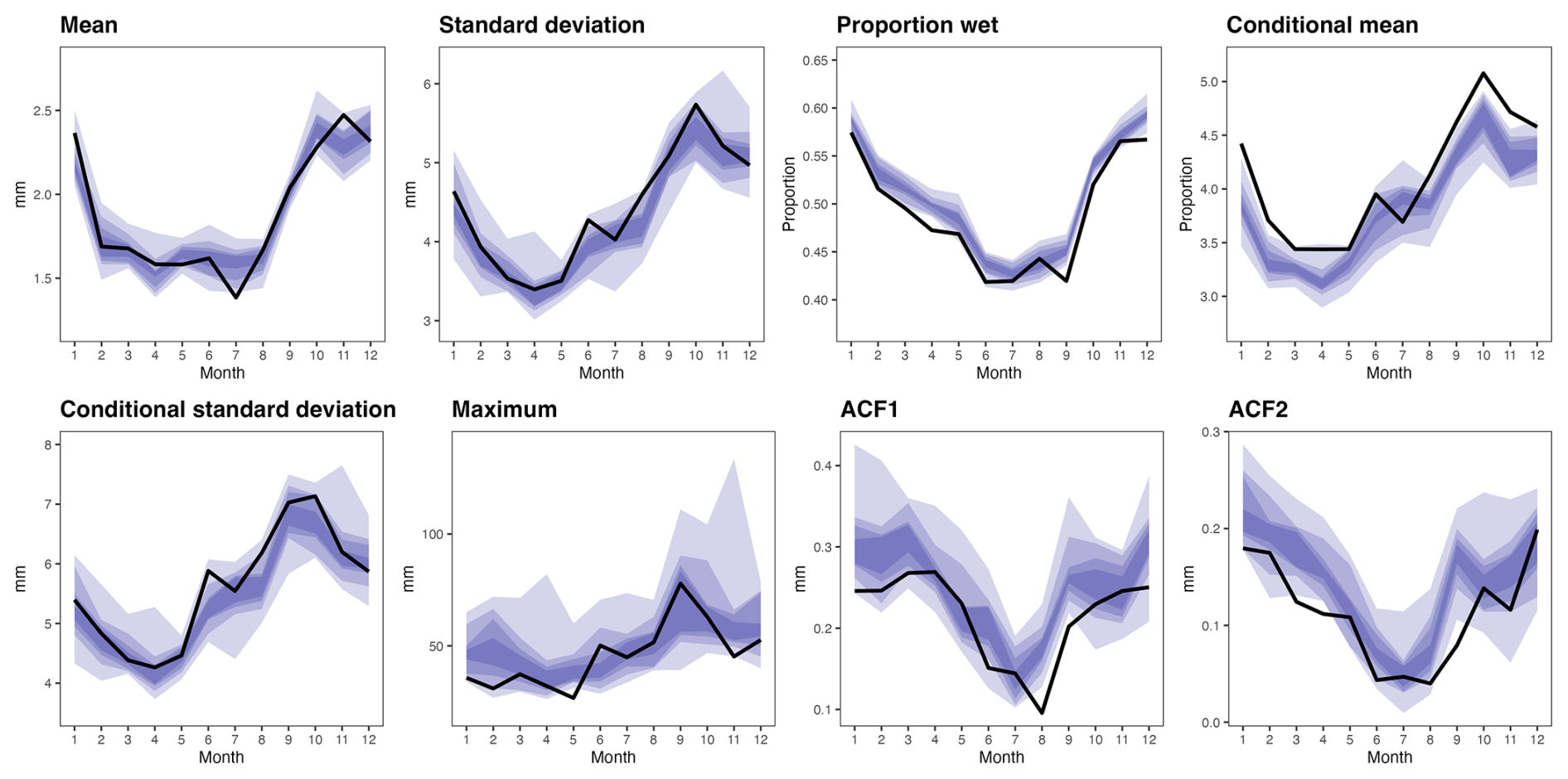
Table 1 Overview of the modelling approach for both parametric and semi-parametric GLMs and GAMLSS

3 Methods

This section provides a brief summary of the GLM-based approach to daily precipitation modelling, and then describes the extensions that are the main contribution of the present paper. For more details of GLMs in this context, see Chandler (2020) and references therein. Table 1 provides a high-level overview of the modelling approaches.

3.1 GLMs for daily precipitation

As noted in Sect. 1, the standard GLM-based approach treats occurrence and intensity separately. Specifically, if the random variable Y_i represents the (possibly thresholded – see above) precipitation intensity for the ith case in a dataset, then the probability of a “wet” day is modelled using logistic regression:

$$\begin{array}{}\text{(1)}& \begin{array}{rl}P(Y_i>\mathrm{0})=& {\mathit{\pi }}_i,\text{ say},\\ & \text{with }\log \left({\displaystyle \frac{{\mathit{\pi }}_i}{\mathrm{1}-{\mathit{\pi }}_i}}\right)={\mathit{x}}_i^{\left(\mathit{\pi }\right)}{\mathit{\beta }}^{\left(\mathit{\pi }\right)}={\mathit{\eta }}_i^{\left(\mathit{\pi }\right)},\text{say}.\end{array}\end{array}$$

Here, ${\mathit{x}}_i^{\left(\mathit{\pi }\right)}$ is a row vector of covariates and β^(π) is a corresponding column vector of coefficients: given these values, the probability of precipitation can be calculated as ${\mathit{\pi }}_i=[\mathrm{1}+\exp (-{\mathit{\eta }}_i^{\left(\mathit{\pi }\right)}){]}^{-\mathrm{1}}$.

If Y_i>0 (corresponding to a “wet” day), then the precipitation intensity is modelled as being drawn from a gamma distribution with mean μ_i (say) and shape parameter ψ. The mean is linked to another covariate vector ${\mathit{x}}_i^{\left(\mathit{\mu }\right)}$, as

$$\begin{array}{}\text{(2)}& \log {\mathit{\mu }}_i={\mathit{x}}_i^{\left(\mathit{\mu }\right)}{\mathit{\beta }}^{\left(\mathit{\mu }\right)}={\mathit{\eta }}_i^{\left(\mathit{\mu }\right)},\text{ say},\end{array}$$

so that ${\mathit{\mu }}_i=\exp \left[{\mathit{\eta }}_i^{\left(\mathit{\mu }\right)}\right]$. The shape parameter ψ is not linked to covariates, however: it is common to all cases, which implies that the standard deviations ({σ_i}, say) of the distributions are proportional to their means with ${\mathit{\sigma }}_i={\mathit{\mu }}_i/\sqrt{\mathit{\psi }}$. This is analogous to the assumption of a constant residual variance in linear regression models.

The covariate vectors ${\mathit{x}}_i^{\left(\mathit{\pi }\right)}$ and ${\mathit{x}}_i^{\left(\mathit{\mu }\right)}$ in Eqs. (1) and (2) need not be the same, although both of them typically include a “1” representing a constant term (so that the corresponding elements of β^(π) and β^(μ) are analogous to the intercepts in linear regression models), as well as quantities representing seasonal and regional variation, transformations of previous days' precipitation (accounting for temporal dependence in precipitation sequences) and indices of large-scale atmospheric structure. Interaction terms can also be included in situations where some covariates may modulate the effects of others – for example, in the case study of Sect. 2 one might reasonably anticipate temporal dependence to be weaker in summer than in winter, due to the seasonally-varying proportion of convective versus frontal precipitation events.

The coefficient vectors β^(π) and β^(μ) can be estimated from a dataset y:=(y₁…y_n)^T, containing daily precipitation observations together with the corresponding covariate vectors $\mathit{\left\{}{\mathit{x}}_i^{\left(\mathit{\pi }\right)}\mathit{\right\}}$ and $\mathit{\left\{}{\mathit{x}}_i^{\left(\mathit{\mu }\right)}\mathit{\right\}}$. This estimation is typically done using maximum likelihood, under the assumption that the associated random variables {Y_i} are conditionally independent of each other given the covariates. In this case, standard theory (and software output) also provides estimated standard errors for the coefficient estimates: these provide a way to determine whether the effect of each covariate is estimated sufficiently precisely to justify its inclusion in a model. By placing priors on the model parameters, Bayesian estimation might also be possible, as for example in Groenke et al. (2026). This potentially allows parameter uncertainty to be propagated into the synthetic sequences produced using the fitted models. However, given the large datasets used for estimation, the effect of parameter uncertainty is generally fairly small, particularly compared to the daily precipitation variability of interest.

To choose covariates, an alternative to the inspection of standard errors is to add additional terms to an existing model and determine whether they lead to a sufficiently large increase in log-likelihood. This can be done either using a likelihood ratio test or by choosing the model with the smallest value of a quantity such as the Akaike Information Criterion (AIC). For a model with generic coefficient vector θ:=(θ₁…θ_k)^T, AIC is defined as

$$\begin{array}{}\text{(3)}& \mathrm{AIC}=-\mathrm{2}\log L({\widehat{\mathit{\theta }}}_y;\mathit{y})+\mathrm{2}k,\end{array}$$

where $\log L({\widehat{\mathit{\theta }}}_y;\mathit{y})$ is the log-likelihood constructed using the data y and evaluated at the maximum likelihood estimate, ${\widehat{\mathit{\theta }}}_y$ say, of θ (the reason for the notation will become clear below). By this criterion, a “good” model is one with a high log-likelihood (and hence a good fit to the data) despite having a small number k of parameters: for further justification of the precise definition, see the Supplement.

The use of likelihood ratio tests or AIC-type comparisons allows a structured approach to model-building in which simple models are gradually extended by adding related groups of covariates, at each stage evaluating the expanded model using a combination of formal comparisons and less formal model diagnostics, such as residual plots, that are designed to assess whether the modelling assumptions are broadly satisfied: see Chandler (2020). However, the associated calculations are valid only under the conditional independence assumption underpinning the calculation of the (log-)likelihoods themselves. For the analysis of data from a single spatial location this assumption can be justified providing the covariate vectors contain appropriate information on previous days' precipitation values (Chandler et al., 2007), but it is usually unrealistic in a multisite context: in the case study of Sect. 2 for example, large-scale frontal weather systems are likely to affect most or all sites simultaneously. To account for the resulting dependence, in a multisite context the standard errors and likelihood ratio tests can be adjusted as described in Chandler and Bate (2007). The AIC can be adjusted similarly (see the Supplement), as

$$\begin{array}{}\text{(4)}& {\mathrm{AIC}}_{\text{adj}}=\mathrm{2}\left[-\log L({\widehat{\mathit{\theta }}}_y;\mathit{y})+\text{ trace }\left({\mathbf{GH}}^{-\mathrm{1}}\right)\right],\end{array}$$

where H is the negative Hessian matrix of the log-likelihood at its maximum and G is the covariance matrix of the gradient vector there: both of these quantities also feature in the adjustments to standard errors and likelihood ratio tests, and can be estimated straightforwardly as by-products of the usual algorithm for maximising the log-likelihood for a GLM. The quantity Eq. (4) is sometimes called the network information criterion or NIC (e.g. Davison, 2003, Sect. 4.7). In passing, we note that these adjustments to standard errors, likelihood ratio tests, and AIC can also be applied in the absence of inter-site dependence and, in this case, all reduce to the “usual” definitions that apply when the log-likelihood is specified correctly because G=H in this case.

Having selected appropriate sets of covariates, estimated the coefficient vectors β^(π) and β^(μ) and carried out diagnostic checks on the fitted model, synthetic precipitation sequences can be generated one day at a time, first by sampling the wet/dry status of each site according to the probabilities defined by the occurrence model Eq. (1) and then, for wet sites, sampling their intensities from the corresponding gamma distributions. In a multisite setting, the generation of realistic sequences requires that the sampling is done in such a way as to respect the inter-site dependence structure: for example, on days when one location experiences precipitation, it is likely that neighbouring locations will also be wet. Inter-site dependence in occurrence and intensity is usually handled separately. For occurrence, Yang et al. (2005b) modelled the distribution of the number of wet sites (on the grounds that in a small region the sites are usually either all wet or all dry) in such a way as to be consistent with the wet-day probabilities determined by the GLM; while, for application to larger regions, Ambrosino et al. (2011) used inter-site dependence models based on thresholded latent Gaussian fields, which allow for a decay in the strength of dependence with intersite distance but can be challenging to estimate when the dependence is very strong. Other approaches also exist: for example, Hughes et al. (1999) use a non-homogeneous hidden Markov model, accounting for spatial dependence directly in the model. Inter-site dependence in intensities is more straightforward and, for GLM-based approaches, is usually achieved via a Gaussian geostatistical model for the Anscombe residuals which are defined in such a way as to have a distribution that is very nearly Gaussian: this approach can also be regarded as corresponding to the use of (approximate) Gaussian copulas (Yang et al., 2005b). Approaches based on latent multivariate Gaussians or latent Gaussian fields have also been used, for example, in Wilks (1998); Kleiber et al. (2012); Keller et al. (2015).

3.2 Extensions: GLMs to GAMLSS

There are two main limitations to GLM-based models for daily precipitation. These are: first, the restriction to linear combinations of covariates in equations Eqs. (1) and (2); and second, the assumption of the constant shape parameter ψ in the gamma distributions for precipitation intensity. The GAMLSS framework of Rigby and Stasinopoulos (2005) can potentially address both of these issues. A summary is provided here: Stasinopoulos et al. (2017) and Stasinopoulos et al. (2024) give further details.

In GAMLSS, the linearity assumption is relaxed by allowing smooth functions of covariates as well as linear combinations. Thus the respective equivalents of Eqs. (1) and (2) are, in their simplest forms,

$$\begin{array}{}\text{(5)}& \begin{array}{rl}\log \left({\displaystyle \frac{{\mathit{\pi }}_i}{\mathrm{1}-{\mathit{\pi }}_i}}\right)=& {\mathit{x}}_i^{(\mathit{\pi },\mathit{\beta })}{\mathit{\beta }}^{\left(\mathit{\pi }\right)}+s_{\mathrm{1}}^{\left(\mathit{\pi }\right)}\left(x_i^{(\mathit{\pi },\mathrm{1})}\right)+\mathrm{\dots }\\ & +s_{M_{\mathit{\pi }}}^{\left(\mathit{\pi }\right)}\left(x_i^{(\mathit{\pi },M_{\mathit{\pi }})}\right)\end{array}\end{array}$$

and

$$\begin{array}{}\text{(6)}& \begin{array}{rl}\log {\mathit{\mu }}_i=& {\mathit{x}}_i^{(\mathit{\mu },\mathit{\beta })}{\mathit{\beta }}^{\left(\mathit{\mu }\right)}+s_{\mathrm{1}}^{\left(\mathit{\mu }\right)}\left(x_i^{(\mathit{\mu },\mathrm{1})}\right)+\mathrm{\dots }\\ & +s_{M_{\mathit{\mu }}}^{\left(\mathit{\mu }\right)}\left(x_i^{\left(\mathit{\mu },M_{\mathit{\mu }}\right)}\right).\end{array}\end{array}$$

In each of these expressions, ${\mathit{x}}_i^{(\ast ,\mathit{\beta })}$ is a row vector of covariates with effects that are represented linearly as before, with coefficient vector β^(∗) (the asterisk “^∗” denoting either “π” or “μ” as appropriate). The terms $s_{\mathrm{1}}^{(\ast )}\left(x_i^{(\ast ,\mathrm{1})}\right),\mathrm{\dots },s_{M_{\ast }}^{(\ast )}\left(x_i^{(\ast ,M_{\ast })}\right)$ are smooth functions of the covariates $x_i^{(\ast ,\mathrm{1})},\mathrm{\dots },x_i^{(\ast ,M_{\ast })}$, which are typically represented semiparametrically using flexible collections of spline basis functions that allow for the data-driven representation of nonlinear effects. Various families of spline basis are available, although our experience is consistent with the received wisdom that the precise choice is relatively unimportant. With one exception, the results reported below use cubic splines Wood (2017, Chapter 5) as implemented in the gamlss (Stasinopoulos et al., 2017) and bamlss (Umlauf et al., 2018) packages in the R programming environment (R Core Team, 2025). The exception is the representation of seasonal effects, for which cyclic splines are used to represent the repeating seasonal cycle – again, as implemented in the cited software.

As written, Eqs. (5) and (6) do not allow explicitly for smooth functions of more than one covariate, or for situations in which the linear coefficient of one covariate (i.e. the corresponding element of β^(∗)) varies smoothly with the value of another so that (e.g.) ${\mathit{\beta }}_j^{(\ast )}:={\mathit{\beta }}_j^{(\ast )}\left(x_k\right)$ in an obvious notation. The representation of systematic regional variation is a canonical situation in which one might wish to consider two covariates (i.e. latitude and longitude) simultaneously: in this case, a bivariate spline basis of the two covariates can be specified, either as a tensor product or as a thin-plate spline Wood (2017, Chapter 5), the latter of which is used in this work. These constructions are all implemented in the gamlss and bamlss software packages, as are the mixed linear-spline terms required for situations where ${\mathit{\beta }}_j^{(\ast )}$ varies smoothly with x_k.

To relax the assumption of a constant shape parameter, GAMLSS allow both the mean and standard deviation (as well as, in principle, the skewness and kurtosis) of a distribution to depend explicitly on covariates. Thus, instead of the simple relationship ${\mathit{\sigma }}_i={\mathit{\mu }}_i/\sqrt{\mathit{\psi }}$ in a gamma GLM for daily precipitation intensity, GAMLSS represent the standard deviations as

$$\begin{array}{}\text{(7)}& \log {\mathit{\sigma }}_i={\mathit{x}}_i^{(\mathit{\sigma },\mathit{\beta })}{\mathit{\beta }}^{\left(\mathit{\sigma }\right)}+s_{\mathrm{1}}^{\left(\mathit{\sigma }\right)}\left(x_i^{(\mathit{\sigma },\mathrm{1})}\right)+\mathrm{\dots }+s_{M_{\mathit{\sigma }}}^{\left(\mathit{\sigma }\right)}\left(x_i^{(\mathit{\sigma },M_{\mathit{\sigma }})}\right).\end{array}$$

In the work reported here, the gamma distributional assumption for wet-day rainfall intensities is retained so that the implied shape parameter for the ith case in the dataset is ${\mathit{\psi }}_i={\mathit{\mu }}_i^{\mathrm{2}}/{\mathit{\sigma }}_i^{\mathrm{2}}$. The complete structure of the daily precipitation sequence at a single location is therefore determined by the three equations Eqs. (5)–(7).

The increased flexibility of GAMLSS compared with GLMs comes at a price: given sufficiently rich collections of splines, almost any model can be made to fit a dataset almost perfectly, simply by specifying very “wiggly” functions $\mathit{\left\{}{s}_j^{(\ast )}\right(\cdot \left)\mathit{\right\}}$ that (almost) interpolate the observations. Techniques such as maximum likelihood estimation therefore tend to yield model fits that are over-optimised to the data at hand and, consequently, are unsuitable for exploring potential variation beyond what has been observed (which, fundamentally, is the purpose of a precipitation generator). To overcome this, GAMLSS are usually fitted by maximising a penalised log-likelihood of the form

$$\begin{array}{}\text{(8)}& \log L({\widehat{\mathit{\theta }}}_y;\mathit{y})-P:=\log L_{\text{PEN}}({\widehat{\mathit{\theta }}}_y;\mathit{y}),\text{ say},\end{array}$$

in which the “penalty” P is typically constructed using the integrated squared second derivatives of the functions $\mathit{\left\{}{s}_j^{(\ast )}\right(\cdot \left)\mathit{\right\}}$. The rationale for this is that the second derivatives measure curvature: wiggly functions have large integrated squared second derivatives, so that the penalty discourages wiggly model fits.

Equation (8) represents a compromise in model fitting: the $\log L({\widehat{\mathit{\theta }}}_y;\mathit{y})$ term encourages fidelity to the available observations, while the penalty P rewards models in which the functions $\mathit{\left\{}{s}_j^{(\ast )}\right(\cdot \left)\mathit{\right\}}$ are smooth. The tradeoff between these two criteria is determined via smoothing parameters for each of the $\mathit{\left\{}{s}_j^{(\ast )}\right(\cdot \left)\mathit{\right\}}$ which, in principle, must be chosen by the analyst. In practice, however, most modern software packages (including the gamlss and bamlss packages used here) incorporate automated, data-driven smoothing parameter selection, essentially by treating the smoothing parameters as auxiliary quantities to be estimated as described in Rigby and Stasinopoulos (2014).

3.3 Model selection with multisite GAMLSS

GAMLSS do not have to include semiparametric terms: parametric GAMLSS for precipitation intensity would retain just the linear components of Eqs. (6) and (7). In this case, as for GLMs, model selection can be done using likelihood ratio tests and AIC-type comparisons, with AIC_adj (defined in Eq. 4) used to account for inter-site dependence where necessary.

For semiparametric models, however, the situation is more complicated. This is partly because AIC requires that models are fitted by maximising a log-likelihood rather than a penalised log-likelihood – although, in principle (see Supplement), a criterion such as AIC_adj is applicable more broadly. In practice, however, the matrices G and H in Eq. (4) must be estimated from the data and, if they are large, sampling errors in their estimation can compromise the accuracy of any associated inference: Jesus and Chandler (2011) give an example of this effect. Semiparametric GAMLSS usually employ large numbers of spline basis functions for each smooth term. For these models therefore, the corresponding matrices G and H are themselves large and Eq. (4) cannot be estimated accurately.

For the semi-parametric GAMLSS we therefore use an alternative model selection criterion, which avoids this difficulty: the WIC (Ishiguro et al., 1991; Shibata, 1997). The underlying motivation is the same as that for AIC and AIC_adj, but WIC uses resampling and does not depend on poorly-estimated quantities. Specifically, let {y^∗} be a collection of resampled datasets that can each be regarded as drawn from the same joint distribution as the observations y (see below). Then, in the current context, WIC is defined as

$$\begin{array}{}\text{(9)}& \begin{array}{rl}\mathrm{WIC}=& -\mathrm{2}\log L_{\text{PEN}}({\widehat{\mathit{\theta }}}_y;\mathit{y})\\ & +\mathrm{2}\left[{\stackrel{\mathrm{‾}}{\log L}}_{\text{PEN}}\left({\widehat{\mathit{\theta }}}_{y^{\ast }};{\mathit{y}}^{\ast }\right)-{\stackrel{\mathrm{‾}}{\log L}}_{\text{PEN}}\left({\widehat{\mathit{\theta }}}_{y^{\ast }};\mathit{y}\right)\right],\end{array}\end{array}$$

where ${\stackrel{\mathrm{‾}}{\log L}}_{\text{PEN}}(\cdot ;\cdot )$ denotes an average of penalised log-likelihoods computed over the resampled datasets.

In Eq. (9), the “adjustment” in square brackets is a difference of two terms. The first is an average of maximised penalised log-likelihoods for each of the resampled datasets; the second, however, is an average of penalised log-likelihoods for the observations y, but evaluated at each of the resample-based estimates ${\widehat{\mathit{\theta }}}_{y^{\ast }}$. The WIC thus aims to compensate for the extent to which the penalised log-likelihood $\log L_{\text{PEN}}({\widehat{\mathit{\theta }}}_y;\mathit{y})$ is likely to be overoptimistic as a performance measure in alternative datasets generated from the same distribution as the observations y. The Supplement gives further details.

The WIC requires that the resampled datasets {y^∗} can be regarded as drawn from the same distribution as the observations y. Standard bootstrap resampling – sampling individual observations with replacement – is not appropriate for multisite precipitation data, because it destroys the inter-site and temporal dependence structure present in each day's observations. Thus alternative resampling approaches are required: Appendix B describes the approach used here. Broadly the idea is to resample individual days instead of individual observations, whilst using additional stratification and adjustments in order to account for covariate dependence, handle missing observations and to ensure that resampled datasets have the same structure as the original one: specifically ensuring that both the full datasets and their dry and wet subsets contain the same number of observations and days with recorded values as the original dataset.

Finally, other resampling-based model selection criteria have been proposed, for example, by Cavanaugh and Shumway (1997) whose criterion is asymptotically equivalent to the WIC (Shibata, 1997). The work reported below uses WIC; we have also examined the Cavanaugh-Shumway criterion and found that it yields very similar conclusions.

3.4 Generating synthetic sequences: revisiting inter-site dependence

GAMLSS can be used to produce synthetic multisite precipitation sequences in the same way as was described for GLMs in Sect. 3.1, using models Eqs. (5)–(7) to determine the daily occurrence probabilities and intensity distributions and with similar adjustments for capturing inter-site dependence. However, as outlined in Sect. 1, there is potential to improve on these options by considering dependence in occurrence and intensities simultaneously when simulating multisite precipitation.

To address this issue, in a similar spirit to Bárdossy and Plate (1992) we use transformed Gaussian fields or, equivalently, Gaussian copulas (Nelsen, 2006; Schölzel and Friederichs, 2008). Denoting by Y_t:=(Y_1t…Y_St)^T the random vector representing precipitation at S sites on day t of a simulation, the elements of Y_t are constructed from a corresponding vector Q_t:=(Q_1t…Q_St) of standard normal random variables with covariance matrix Σ, as

$$\begin{array}{}\text{(10)}& Y_{\text{st}}=\left\{\begin{array}{ll}\mathrm{0}& \text{if }\mathrm{\Phi }\left(Q_{\text{st}}\right)<\mathrm{1}-{\mathit{\pi }}_{\text{st}}\\ F_{\text{st}}^{-\mathrm{1}}\left(\frac{\mathrm{\Phi }\left(Q_{\text{st}}\right)-(\mathrm{1}-{\mathit{\pi }}_{\text{st}})}{{\mathit{\pi }}_{\text{st}}}\right)& \text{otherwise}.\end{array}\right.\end{array}$$

Here, π_st is the probability of non-zero precipitation as obtained from the occurrence model Eq. (5); $F_{\text{st}}^{-\mathrm{1}}(\cdot )$ is the inverse cumulative distribution function (CDF) of the gamma distribution for wet-day amounts defined by Eqs. (6) and (7); and Φ(⋅) is the CDF of the standard normal distribution. It is easily verified that under Eq. (10), $P(Y_{\text{st}}>\mathrm{0})={\mathit{\pi }}_{\text{st}}$ and $P(Y_{\text{st}}\le y|Y_{\text{st}}>\mathrm{0})=F_{\text{st}}(y)$ so that the procedure yields precipitation with the correct marginal (i.e. site-specific) distributions at each site.

The first line of Eq. (10) – yielding a simulated dry day – corresponds to a situation in which Q_st is censored, meaning that its precise value is unknown: it is only known not to exceed ${\mathrm{\Phi }}^{-\mathrm{1}}(\mathrm{1}-{\mathit{\pi }}_{\text{st}})$. The {Q_st} can be regarded as normalised quantile residuals (Dunn and Smyth, 1996), censored on dry days. There is, moreover, a connection with existing representations of inter-site dependence in precipitation intensities: if π_st=1 so that the first condition in Eq. (10) is never met, then the transformation in the second line is similar in spirit to the use of transformed Anscombe residuals for this purpose by Yang et al. (2005b). The current proposal can therefore be seen as a natural extension of, and a way of linking, apparently distinct approaches from the literature.

Under Eq. (10), inter-site dependence in the precipitation Y_t is induced by the covariance matrix Σ of the Gaussian random vector Q_t. In particular, if Σ is the identity matrix, then Q_t contains independent standard normal random variables, and Eq. (10) produces independent precipitation values from the combined occurrence/intensity model at each site. To generate realistic multi-site precipitation sequences, however, non-zero off-diagonal elements of the matrix Σ must usually be estimated from the data y. Following standard practice for GLM-based precipitation generators, this is done after fitting the marginal occurrence and intensity models Eqs. (5)–(7): thus, when estimating Σ, the quantities {π_st}, {μ_st} and {σ_st} are considered known.

In most situations involving more than a few sites, estimation of Σ is complicated by the fact that there are typically few, if any, periods during which data from all sites are simultaneously available. This can be handled (e.g. Wilks, 1998) by estimating correlations separately for each pair of sites using all dates for which both are operational. The resulting matrix of inter-site correlations is not guaranteed to be positive definite however: to address this, we subsequently fit a spatial correlation model to the pairwise estimates. This ensures a valid correlation matrix, and also provides correlations for pairs of locations with non-overlapping records or that are ungauged. We use a Matérn correlation function for this purpose, due to its flexibility in capturing a wide range of correlation behaviours (Porcu et al., 2024). According to this model, the residual correlation between two locations separated by a distance d>0 is

$$\begin{array}{}\text{(11)}& C_{\mathit{\nu }}\left(d\right)=\mathit{\alpha }{\displaystyle \frac{{\mathrm{2}}^{\mathrm{1}-\mathit{\nu }}}{\mathrm{\Gamma }\left(\mathit{\nu }\right)}}{\left(\sqrt{\mathrm{2}\mathit{\nu }}{\displaystyle \frac{d}{\mathit{\rho }}}\right)}^{\mathrm{2}}{K}_{\mathit{\nu }}\left(\sqrt{\mathrm{2}\mathit{\nu }}{\displaystyle \frac{d}{\mathit{\rho }}}\right),\end{array}$$

where Γ(⋅) is the Gamma function and K_ν(⋅) the modified Bessel function of the second kind. The form of the correlations is determined by the two parameters ν, ρ, and α, respectively controlling the smoothness of the residual fields, the distance-dependent rate of correlation decay, and the “nugget” effect representing the limiting correlation at small non-zero distances (Andrianakis and Challenor, 2012). In the work reported below, the parameters are estimated from the pairwise inter-site correlations using weighted least squares, weighting the correlation between each pair of sites according to the number of days' data from which it was calculated. This weighting ensures that the correlation model fit is not influenced unduly by pairwise correlations that are estimated imprecisely.

For schemes that treat dependence in occurrence and intensities separately, separate correlation models are needed for each component. For intensities, the pairwise correlations to which Eq. (11) is fitted can be calculated directly from the relevant (transformed) residuals (e.g. Yang et al., 2005b); while those for occurrence can be inferred from the proportion of days for which both sites are simultaneously wet (e.g. Ambrosino et al., 2014). For the combined occurrence/intensity scheme Eq. (10), however, a single correlation model is needed, and neither of these approaches is feasible, because there are invariably days for which one site in a pair is wet while the other is dry. We thus estimate the pairwise correlations using maximum likelihood as described in Appendix C: although this requires numerical optimisation for each pair of sites, it is a principled approach that is generally applicable and can in theory extend beyond bivariate estimation.

Having estimated the correlation matrix Σ, synthetic multisite precipitation sequences can be generated one day at a time: on day t of simulation a vector Q_t of standard normal variates with correlation matrix Σ is simulated, and then converted to a corresponding precipitation vector Y_t via the transformation Eq. (10).

4 Application to the Blackwater catchment

It is of interest to determine whether GAMLSS offer improved performance compared with GLMs when generating synthetic precipitation sequences; and, if so, whether the improvement is due to the use of semiparametric rather than parametric covariate effects or to the use of a non-constant shape parameter in the intensity model (or both). To explore these questions, we compare the performance of four precipitation generators fitted to the Blackwater data from Sect. 2. The first of these uses GLMs, with a parametric representation of covariate effects in both occurrency and intensity models and a constant shape parameter in the latter; while the second is a GAM (see Sect. 1) allowing a semiparametric representation of covariate effects and which, for present purposes, can be regarded as a special case of a GAMLSS in which the covariates influence only the location parameter of the intensity distribution. These models are then extended, respectively to parametric and semiparametric GAMLSS, allowing both the location and scale parameter of the intensity distribution to depend on covariates. This approach, starting with and then extending “location-only” models, follows the “parameter-hierarchy” recommended in Stasinopoulos et al. (2017).

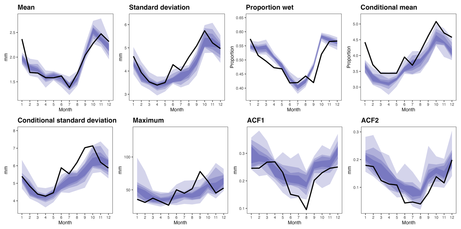
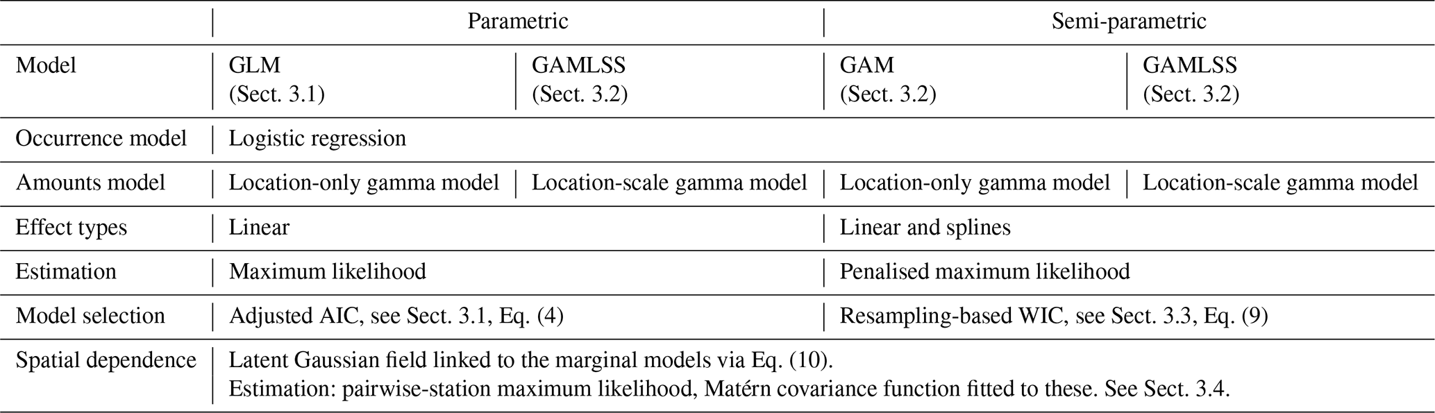
Figure 2 Monthly summary statistics for 16-site average daily precipitation series. The black line shows the observed values, whilst the blue shaded areas correspond to intervals containing, respectively 30 %, 50 %, 70 % and 90 % of the distribution of simulation-derived values from the parametric GLM. Statistics: monthly mean, monthly standard deviation, proportion of wet days, conditional mean (mean on rainy days), conditional standard deviation (standard deviation on rainy days), monthly maximum, autocorrelation at lag 1, autocorrelation at lag 2.

4.1 Model-building strategy

Each model is constructed using a structured approach (Chandler, 2005). The parametric GLM and semiparametric GAM are constructed independently of each other, in each case starting with a simple baseline model and successively adding terms in perceived order of importance; see Appendix D. The final GLM and GAM for precipitation intensity are then taken as starting points for the modelling of intensity standard deviations in the respective GAMLSS. Throughout, multiple effect forms (i.e. parametric forms and/or spline specifications) for potential covariates as well as interactions (see Sect. 3.1) are tested; and alternative formulations are compared using the adjusted AIC (4) and WIC (9), respectively for the parametric and semiparametric models. For the semi-parametric models always both parametric and spline-based effects are tested. To represent seasonal variation, sine and cosine functions of the day of the year are used in the parametric models; and cyclic splines in the semiparametric ones. Systematic regional variation is captured using functions of latitude, longitude, and altitude. For the parametric models, latitude–longitude effects are represented by Legendre polynomials; for the semiparametric models, a thin-plate bivariate spline in latitude and longitude is used instead. Following Yang et al. (2006), the change in measurement resolution (see Sect. 2) is accounted for via a binary covariate taking the value 0 for all observations before 1970 and 1 for all subsequent observations: the effect is to provide an adjustment within the models for any systematic changes arising from the coarser resolution of the data in the early part of the record, thus avoiding the need for data preprocessing that may have unintended consequences (see Appendix A).

After model selection, standard checks on residuals Stasinopoulos et al. (2017, Chapter 12) are carried out as an initial assessment that the models appear to capture most of the systematic structure in the data, before carrying out more extensive tests via simulation (see next section). Finally, for each of the four options (GLM, GAM, parametric and semiparametric GAMLSS) a residual correlation matrix Σ is estimated as described in Sect. 3.4, for use in the inter-site dependence model Eq. (10).

4.2 Simulation settings

The performance of each precipitation generator is assessed by comparing statistics of the observed data over the period 1959–2022 with those for each of 19 simulated sequences over the same period. The number of simulations is limited by the computation time for the GAMLSS as implemented in the bamlss package: this is discussed further in Sect. 5 below. Each statistic is calculated separately for every simulated sequence, thus yielding a distribution of 19 values: if the precipitation generator is realistic, then the corresponding statistic computed from observations should lie within the range of this distribution 90 % of the time on average, since it has a $\mathrm{1}/\mathrm{20}$ chance of being less (resp. greater) than the minimum (resp. maximum) from the simulations.

Each simulation is initialised with the first three observed days at each station. Simulations are carried out only on days and at stations where observations are available. When several consecutive observations are missing for a station, the simulation is reinitialised once new observed values become available, using these as the new lagged inputs. This guarantees a like-for-like comparison of simulations and observations. Much of the subsequent analysis will focus on the subset of 16 stations that report through most of the study period. The observations used for initialisation are not used in the comparison exercise, as the simulations contain no corresponding values.

Figure 3 As Fig. 2 but for the semiparametric GAMLSS.

4.3 Reproduction of key precipitation statistics

For each month of the year, Figs. 2 and 3 compare the observed values of several key summary statistics with those derived from simulations of the parametric GLM and semiparametric GAMLSS (similar figures for the parametric GAMLSS and semi-parametric GAM can be found in the Supplement). These statistics all relate to the daily precipitation series averaged over the 16 stations reporting through most of the 1959–2022 period.

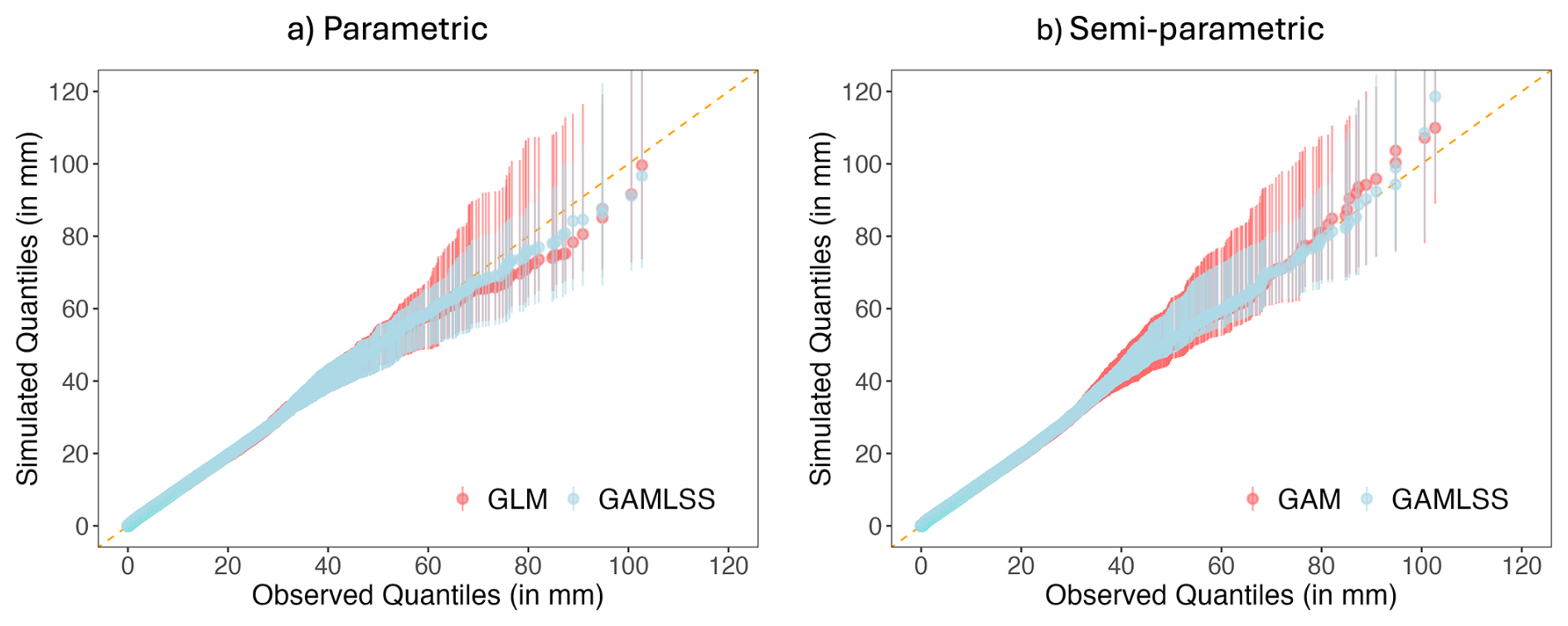
Figure 4 Quantile-quantile plots comparing observed and simulated precipitation distributions for both the parametric (a) and semiparametric (b) location (GLM/GAM, red) and location-scale (GAMLSS, blue) models. Distributions are pooled across all stations and across the entire study period 1959–2022. Vertical lines and points indicate ranges and median values, respectively, from 19 simulations.

In both figures, most of the observed statistics fall within the 90 % range of the simulations: this indicates good performance of both the occurrence and intensity models in the parametric and semi-parametric case. Results for the parametric GAMLSS and semi-parametric GAM are similar (see Supplement). The overall mean is well captured across all models, however, there is some indication that the conditional (i.e. wet-day) mean might be underestimated. The proportion of wet days and the standard deviation statistics (both overall, as well as conditional) seem better captured by the semiparametric GAMLSS, compared to the parametric models. For the proportion of wet days, this is most likely due to the more flexible representation of covariate effects in the GAMLSS framework, since the GAMLSS-based modelling of standard deviations is not used in the occurrence model. By contrast, the improvement in representing the standard deviations is also seen for the parametric GAMLSS (see Supplement), whence this improvement probably comes from the ability to model variation in the shape parameter of the gamma distributions. In the Supplement (Sect. S4 in the Supplement) we further analyse the persistence of dry and wet spells which we find is well reproduced by all four precipitation generators.

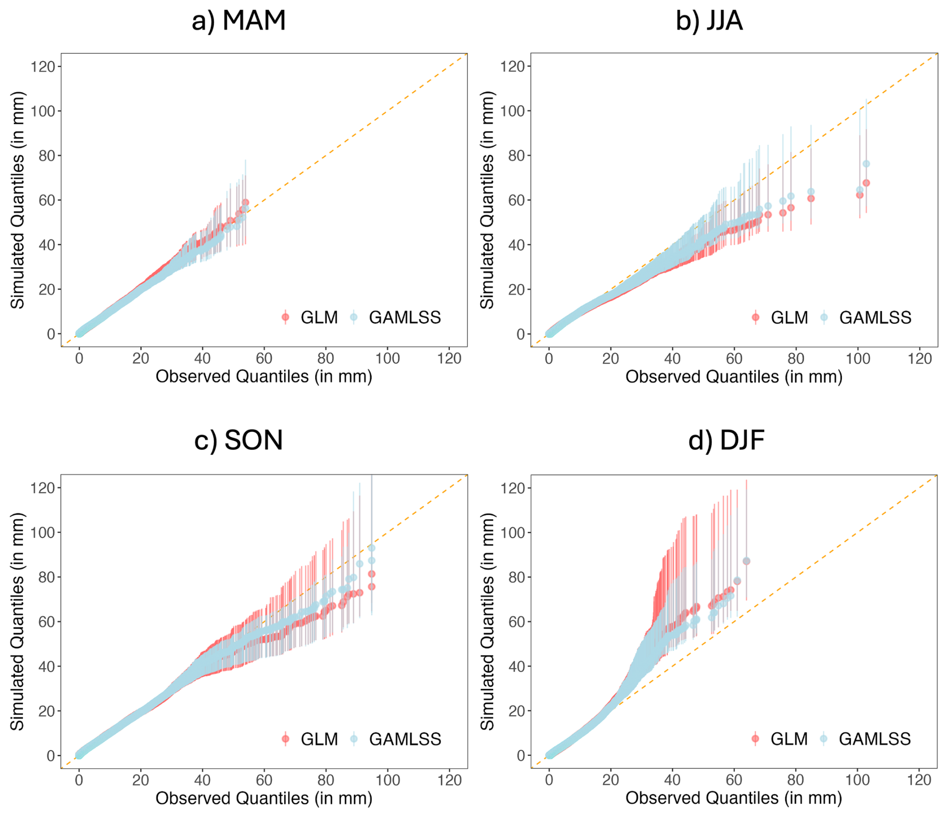
Figure 5 Quantile-quantile plots comparing observed and simulated precipitation distributions values for both the parametric location model (GLM, red) and the parametric location and scale model (GAMLSS, blue) for all four seasons. Distributions are pooled across all stations and across the entire study period 1959–2022. Vertical lines and points indicate ranges and median values, respectively, from 19 simulations.

4.4 Daily precipitation distributions

Next, we focus on the generators' ability to reproduce the distribution of daily precipitation values, both overall and by season. This is done via quantile-quantile plots, in which the ordered values from each simulation (from smallest to largest) are plotted against those from the observations as in Fig. 4. Here, the daily values from all sites throughout the study period are pooled, and each panel shows the results from a location-only model (i.e. a GLM or a GAM) and a location–scale GAMLSS: covariate effects are represented parametrically in Fig. 4a but semiparametrically in Fig. 4b, and each vertical line indicates the range of values across the 19 simulations.

Figure 4 shows that overall, all four generators capture the rainfall distribution well: the ranges of ordered values from the simulations encompass the line of equality, and the medians of the 19 simulated values at each point fall close to this line. The ranges of simulated values are broadly similar for precipitation amounts up to around 50 mm (this is around the 99.96th percentile of the observed distribution); but there are larger differences in the upper tail of the distribution, where the GAMLSS yield less between-run variability, whilst still encompassing the line of equality. These results are also consistent when aggregating precipitation on a weekly scale (not shown).

The good reproduction of the overall precipitation distribution in Fig. 4 is consistent with the GLM-based results of Yang et al. (2005b), who nonetheless found systematic differences between observed and simulated distributions in individual seasons. To investigate this further, therefore, Fig. 5 compares the observed and simulated precipitation distributions from the two parametric precipitation generators (GLM and parametric scale-location GAMLSS) by season. Here, both sets of simulations tend systematically to overestimate the upper tail of the precipitation distribution in winter and, to a lesser extent, to underestimate in summer. The GLM-based result here is similar to that reported by Yang et al. (2005b). Some improvement can be seen for the GAMLSS, where in particular in DJF the amount of overestimation is reduced in some simulations. Nonetheless, the improvement appears relatively small since the medians of the simulated quantiles are similar in the GLM and the GAMLSS.

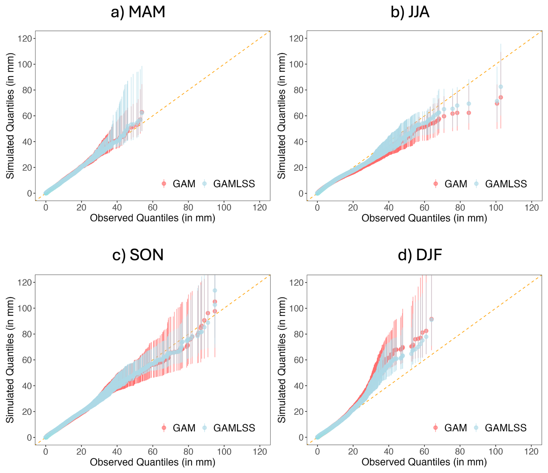
Figure 6 As Fig. 5 but for the semiparametric location (GAM, red) and location scale model (GAMLSS, blue).

Figure 6 shows the corresponding plots for the semi-parametric models. The results are broadly comparable with those in Fig. 5. The semiparametric GAMLSS simulations show again some improvement in Summer and Winter, however, the overall biases are still present. This overall pattern also persists when focusing on individual months rather than entire season: see for example Fig. S3 in the Supplement showing results for January in which, as with the winter comparisons above, the simulations tend to overestimate the upper tail of the distribution; this is slightly less pronounced for the semiparametric GAMLSS than for the other three generators, however.

Taken together, these results suggest that modest improvements in the representation of seasonal precipitation tails can be gained by relaxing the assumption of a constant shape parameter although this does not fully resolve the issue. The more flexible representation of potentially nonlinear covariate effects compared with a standard GLM does not seem to improve tail behaviour much. We note, however, that whilst seasonal tail deviations are apparent in the pooled distribution of single-site rainfall studied above, no such deviation is seen in the distribution of catchment-averaged rainfall for any of the models (see Figs. S4 and S5 in the Supplement). This indicates that for most hydrological applications all weather generator models studied here will have satisfactory performance in terms of extremes, and stands in contrast to the result in Yang et al. (2005b) who found seasonal tail deviations in the time series of average rainfall for GLM-based models. This is probably due either to different treatment of recording resolution (see Appendix A) or to the use of different atmospheric covariates: this work uses ERA5-derived variables, whilst Yang et al. (2005b) used an index of the North Atlantic Oscillation (NAO).

4.5 Distributions of annual maxima

An alternative way to characterise the upper tail behaviour is via extreme value theory (Coles, 2001), which is often used to study the expected frequency of rare events for purposes such as flood risk assessment. In particular, a common summary of potential extremal behaviour is the shape parameter, often denoted as ξ, of a generalized extreme value (GEV) distribution fitted to a collection of annual maxima. If ξ>0, as often reported for daily precipitation (e.g. Katz et al., 2002), then the distribution of extremes is heavy-tailed which implies a potential for as-yet-unobserved extreme events to greatly exceed historical values, whereas if ξ=0 then the distribution is light-tailed, and if ξ<0 then the distribution has a finite upper bound.

To investigate the extremal behaviour of each precipitation generator over the period 1959–2022, the extRemes package (Gilleland and Katz, 2016) is used to fit GEV distributions to the annual maxima of selected time series derived from each simulation: for each series, the mean and standard deviation of the 19 resulting estimates of ξ are compared with the estimate and standard error derived from the corresponding observations. This standard error is based on large-sample theory and aims to approximate the standard deviation of estimates obtained under repeated sampling: thus it should be comparable with the standard deviation of the simulation-based estimates. We follow the advice of Belzile et al. (2023) and standardize the annual maxima prior to fitting: this does not affect the shape of the distribution.

Table 2 Shape parameters of GEV distributions fitted to observed and simulated annual maxima, for selected series of daily precipitation over the period 1959–2022. Simulation-derived estimates are from the semiparametric GAM and GAMLSS. Values in parentheses are standard errors: those for the observation-based estimates are based on large-sample approximations, while those for the simulation-based estimates are the empirical standard deviations across simulations.

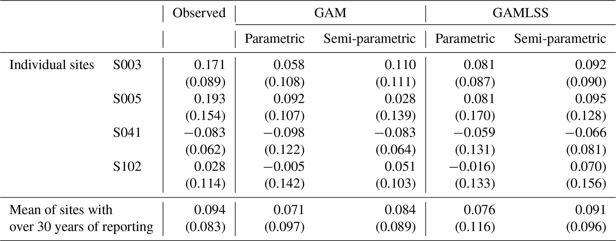
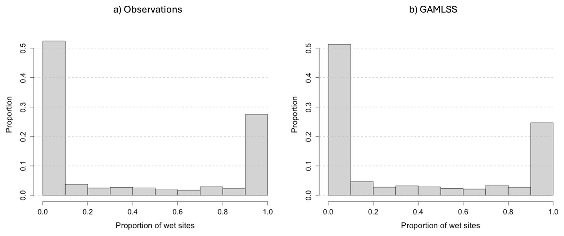
Figure 7 Histograms of the proportion of rainy stations on a given day for the observations (a) and the simulations from the semiparametric GAMLSS (b).

Table 2 reports the results of this exercise for a representative set of time series: for four individual stations, and for the 16-site average. The observation- and simulation-derived estimates are all in good agreement: in particular, the point estimates of ξ are (slightly) positive for most of the considered series. This confirms that the extremal behaviours of the simulations and observations are qualitatively similar, despite the generators not being calibrated directly to reproduce such behaviour.

4.6 Inter-site dependence

In their original study of precipitation in this catchment, Yang et al. (2005b) found that inter-site dependence was extremely strong due to the relatively small size of the area. It is challenging to develop simulation strategies that can capture this, particularly when separate dependence models are used for precipitation occurrence and intensity: correlation-based dependence structures for occurrence are hard to identify in this case, because sites are typically either all wet or all dry on most days. To address this, Yang et al. (2005b) introduced an indirect approach for capturing dependence in precipitation occurrence, based on the distribution of the number of wet sites on each day. It is possible, however, that correlation-based dependence structures can be used for small catchments by modelling dependence in occurrence and intensity simultaneously (e.g. via Eq. 10) because, in this case, correlations learned predominantly from precipitation intensity are implicitly shared with the occurrence model.

To investigate this, we here evaluate the inter-site dependence structure in our simulations. The results presented are produced using the semiparametric GAMLSS; results obtained from the other models are not shown but are similar.

4.6.1 Occurrence

Following from Yang et al. (2005b), we investigate dependence in precipitation occurrence by studying the distribution of the proportion of sites that are wet on each day. Figure 7 shows histograms of this distribution for the observations (Fig. 7a) and simulations (Fig. 7b). Here, the data from all 19 simulations have been pooled to produce a single distribution.

Figure 7a shows that on around 80 % of days in the observations, the proportion of wet sites is either above 0.9 or below 0.1. This corresponds to very strong inter-site dependence as noted above. The simulations reproduce the shape of the histogram well (Fig. 7b), albeit with slightly fewer days (around 76 %) in these outer histogram bins. The difference between the histograms is more pronounced at the right-hand end, where the proportion of wet sites exceeds 0.9 on 27.5 % of days in the observations but 24.6 % in the simulations. This discrepancy is unlikely to be important in many applications: in situations where it is important however, it would be preferable to use an inter-site dependence model, such as that of Yang et al. (2005b), that is specifically designed for this purpose.

4.6.2 Intensity

We next examine inter-site dependence in intensities. The mean Pearson correlation between pairs of stations when both are wet is 0.823 in the observations and 0.815 in the simulations (standard deviation across simulation runs: 0.0072). Across all pairs of stations, the mean absolute difference between observed and simulated correlations is 0.055. This deviation is most likely due to the fact that the Matérn assumption of homogenous correlation decay with distance is not fully realistic due to the small area (see Fig. 7 in the Supplement which shows estimated bivariate correlations against Matérn fitted ones). Overall, the dependence seems slightly underestimated, but generally well captured.

As noted in Sect. 2, precipitation in the study area is mostly associated with large-scale synoptic systems, although localised convective events occur in summer. This suggests the potential for seasonal variation in the strength of inter-site dependence, with localised summer precipitation resulting in weaker dependence. Analysis of the observations confirms this, with average pairwise intensity correlations ranging from 0.75 in summer to 0.87 in winter. This variation is not fully captured in the simulations, although the simulated inter-site correlations are indeed weakest in summer (Table 3).

Table 3 Average correlations between pairs of sites for days when both are wet, 1959–2022. Simulation-based results are derived from the semiparametric GAMLSS; the “original” column uses a constant inter-site correlation matrix, while the “revised” column uses a separate matrix for each season. Figures in parentheses are standard deviations across simulations.

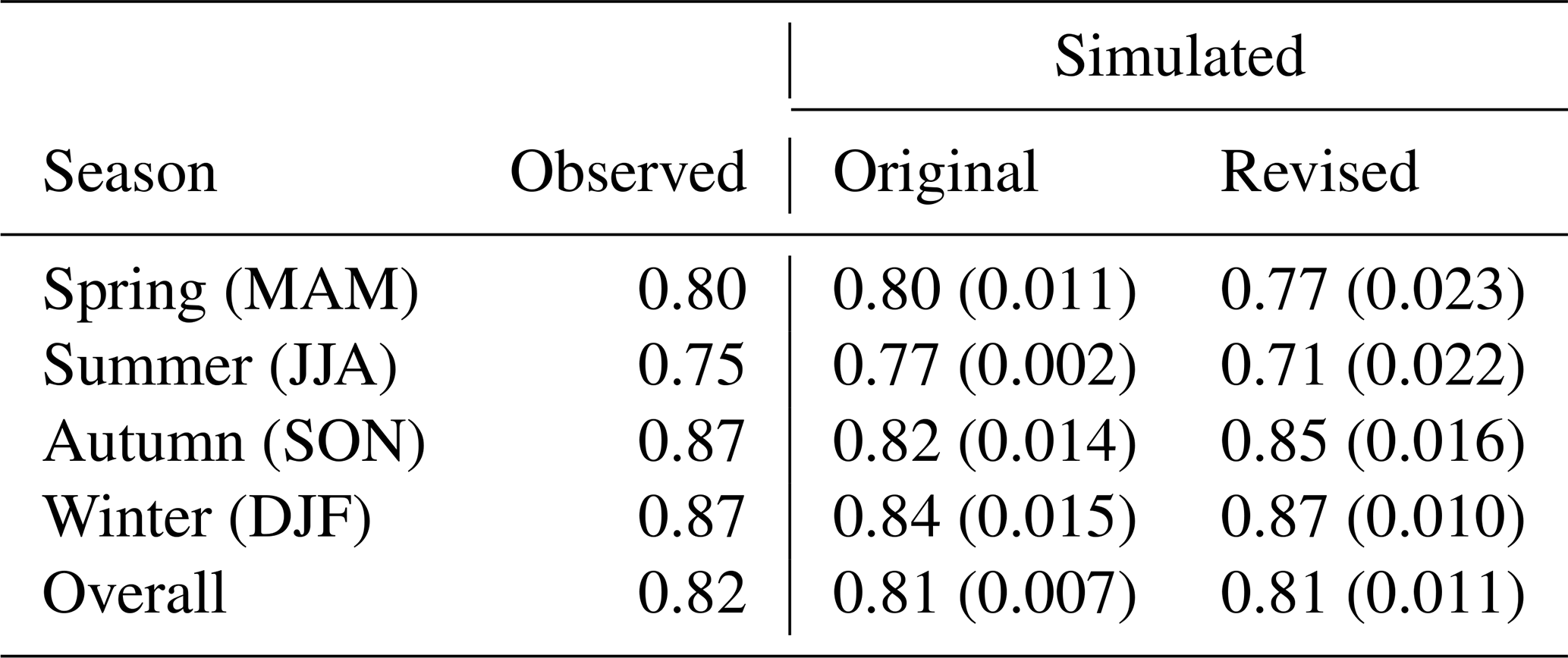
To address this, we experiment with the use of separate Matérn correlation parameter sets for each season. As shown in the final column of Table 3, this produces a small improvement in capturing the Winter and Autumn correlation, but none in Spring and Summer. Further investigation is needed to understand this. One possibility is that there is unmodelled seasonality in the systematic regional variation of precipitation over the catchment: simple interactions between seasonal and spatial variation were not chosen in the AIC and WIC-based model selection, but there may be potential for more complex representations to capture the effects. In addition, when stratifying correlations seasonally the data records for computing bivariate correlations can become quite short, leading to larger estimation uncertainty. And finally, as indicated above, correlations might not always decay homogeneously with distance due to the size of the area which raises questions about the use of the Matérn covariance. In particular, we also find that there is larger variance between the estimated latent bivariate correlations in Summer than in Winter. This will not be captured by the chosen covariance structure.

4.6.3 Intensity-Occurrence cross-dependence

“Spatial intermittence” refers to the dependence between dry sites and sites nearby that might be expected to only record small precipitation amounts. In the Supplement we analyse the distribution of precipitation amounts in the area, for days when at least one station recorded rainfall but the proportion of wet sites did not exceed 50 %. The remaining wet stations usually only record small amounts of rain in that case. We find that spatial intermittence is captured by the dependence template, meaning that it reproduces the shifted distribution of precipitation amounts, conditional on only a small proportion of the catchment being wet.

5 Discussion and conclusions

This work has examined the use of generalized additive models for location, scale and shape (GAMLSS) to extend the class of precipitation generators based on generalised linear models (GLMs). GAMLSS allow greater flexibility in modelling than GLMs, first via spline-based representations of covariate effects and second by relaxing the assumption of a constant shape parameter in the precipitation intensity distribution, instead allowing the shape parameter itself to depend on covariates. This potentially allows for the development of improved generators in applications including flood risk assessment and water resource management: the inclusion of large-scale atmospheric predictors as covariates also renders the models suitable for downscaling climate model outputs (Maraun et al., 2010). In the latter context, however, a potential caveat is that semiparametric models provide data-driven estimates of covariate effects on the parameters of the precipitation distribution – hence, almost by definition, they tend to perform poorly when extrapolating beyond the range of covariates in the training data. This means that the models may not be suitable for downscaling (say) future scenarios in which the large-scale atmospheric predictor configurations differ substantially in terms of data range from those in the historical record. To some extent, this is a caveat of any statistical downscaling method (Maraun and Widmann, 2018): it is perhaps more serious, however, with a semiparametric model that imposes minimal constraints on the estimated covariate effects. Further work is needed to determine how serious a problem this is likely to be in applications.

Although GAMLSS are reasonably well established in the statistical literature, their use as multisite precipitation generators requires the use of estimation and model selection criteria that account for inter-site dependence: we suggest that the adjusted AIC and the WIC can be used for this purpose. A further contribution is the development of an approach, within the GLM/GAMLSS framework, that accounts simultaneously for inter-site dependence in precipitation occurrence and intensity.

In a case study focusing on a small catchment in southern England, we find that GAMLSS-based precipitation generators help improve some of the known deficiencies of GLMs. Introducing a semiparametric representation of covariate effects allows to better capture some precipitation statistics. By relaxing the assumption of the constant shape parameter, GAMLSS slightly improve on GLMs in representing seasonal variation in the upper tail of the precipitation distribution without adversely affecting other aspects of performance – but also without fully addressing the problems. These results suggest that, whilst adjusting the scale parameter and relaxing linearity of covariate effects – our initial hypothesis for the source of the problem – does yield modest improvements, it does not resolve the issue; adequately capturing seasonal tail behaviour may therefore require going beyond the widely-used gamma family itself, rather than adding further flexibility within it. Future work will consider distributions other than the gamma as the basis for an intensity model, perhaps considering three-parameter distributions to provide additional control over tail behaviour. In this work we briefly experimented with the three parameter generalised gamma distribution, which provides an additional shape parameter allowing independent control over tail behaviour. We did not, however, find consistent improvements over the classical gamma distribution and fitting proved less stable. Possibly, however, alternative three or four parameter distributions might yield benefits, for example one might consider the Box-Cox Power exponential (Rigby and Stasinopoulos, 2004). Approaches based on extreme value theory could also be explored (see for example Friederichs, 2010; Huser and Davison, 2014), possibly combined with a gamma model for the main body of the distribution as in Vrac and Naveau (2007). However, whilst the incorrectly captured seasonal tails of the intensity distribution are undesirable from a statistical perspective, the practical consequences of this may be less serious given the fact that the seasonal tails of the areal average intensity distribution are well represented (see Supplement).

In the same case study, inter-site dependence is strong due to the relatively small size of the study area. It is hard to replicate this with the techniques usually used in conjunction with GLMs and related precipitation generators: the approach proposed here builds on ideas from other types of generators. It captures the dependence well overall, albeit slightly underestimating the proportion of days for which all, or almost all, of the area is wet: for applications in which this is problematic, it would be preferable to use a model that is specifically designed to reproduce the distribution of the proportion of wet sites.

A further deficiency of the proposed model – along with other common inter-site dependence models – is that it does not fully capture seasonal variation in the strength of dependence arising, for example, due to the differing prevalence of convective and frontal systems in summer and winter. It is slightly surprising that this problem is not fully resolved via the use of season-specific correlation structures: further investigation of this is needed. Possibilities include expressing parameters of the Matérn covariances (or any other covariance function) as a function of seasonality, or exploring spatial-seasonal interactions within the GLM/GAMLSS itself.

A small but potentially important contribution of this work relates to the treatment of changes in recording resolution over time. Previously, where the issue has been considered at all, it has often been handled by preprocessing the data prior to analysis, for example, by rounding all values to the nearest 0.5 mm. Having discovered that the properties of simulated sequences can be sensitive to the choices made in such a preprocessing step (see Appendix A), we propose instead to address the issue within the models themselves. This is done via the inclusion of binary covariates taking the value 0 for all observations measured to a “reference” resolution (typically the finest available) and 1 for all others: the effect is to allow within the model for any systematic changes that arise from the differences in resolution.

We have not so far discussed the computational cost of the GAMLSS framework. Fitting of the parametric GAMLSS is fast and comparable in terms of speed with the fitting of GLM-based weather generator models as in Rglimclim (Chandler, 2020). Fitting of the semi-parametric models is slower and might take several minutes on a standard laptop (Intel Quad Core i5-1145G7 @ 2.60 GHz CPU, 16 Gb RAM), but can for the most complex models take in the order of 15–30 min. Model selection using the WIC can also be slow for large models, due to the need to refit the model to every bootstrap sample in order to calculate the $\mathit{\left\{}{\widehat{\mathit{\theta }}}_{{\mathit{y}}^{\ast }}\mathit{\right\}}$ in Eq. (9). It would be helpful to investigate or develop alternative model selection criteria that can be used for semiparametric models in the presence of unresolved spatial dependence (or other forms of model mis-specification). Adjusted AIC-based model selection is fast as the required terms are usually obtained as a by-product of the maximum likelihood optimization. Similarly, fitting of the spatial dependence template is efficient and highly parallelizable, but might become restrictive for large station datasets in which case other optimizations might be necessary. Finally, simulation of the parametric and semi-parametric GAMLSS is slow and can take on the order of several hours to generate 50 years of simulated data for all stations. This is due to inefficiencies in the gamlss and bamlss packages, which are not designed for autoregressive simulation. Using specialised software, as in Groenke et al. (2026), this can be sped up strongly to the order of seconds to minutes, however, this comes at the cost of ease-of-implementation of spline-based models.

An open question is to determine whether the results from our Blackwater case study hold more generally. Experience with the use of GLM-based precipitation generators suggests that the conclusions of Yang et al. (2005b), based on data for the same catchment, are indeed generally applicable across a range of climatologies and catchment sizes; and Gaussian copulas have been shown to work well for capturing dependence in precipitation intensity in larger areas (e.g. Kleiber et al., 2012; Ambrosino et al., 2014). Nonetheless, further experience is needed to verify that the more complex GAMLSS methodology is similarly transferable.

Appendix A: Influence of rounding on gamma distribution fits

While carrying out this research, as noted in Sect. 1 we noted that some properties of simulated precipitation sequences were sensitive to decisions made during data preprocessing – notably the handling of inconsistencies in the recording resolution of data used to fit the models. This appendix illustrates the issue.

Inconsistencies in recording resolution are often handled by rounding all records to a common resolution, such as 0.5 or 0.1 mm, prior to model fitting (Ambrosino et al., 2014). It is known that maximum likelihood fits of gamma distributions are sensitive to rounding errors in small values McCullagh and Nelder (1989, Sect. 8.3); however, the effect on the upper tail of the distribution is perhaps less widely appreciated.

We demonstrate this effect by simulating 100 000 values from a gamma distribution with mean 5 and dispersion 1 (these parameter choices are the nearest integers to estimates obtained from the data in our case study). Using maximum likelihood, we then fit a gamma distribution to the simulated data after applying a rounding strategy. Finally we simulate a further 100 000 values from this fitted distribution, apply the same rounding strategy and plot the ordered values of the two rounded datasets against each other in a quantile-quantile plot. This final step provides a like-for-like comparison in determining whether the fitted distribution provides a good match to the data used to fit it, although the results reported below do not change materially if the second dataset is not rounded.

Two rounding strategies are considered, as follows:

Rounding only: round all observations to the nearest 0.5 and remove all values rounded to zero, meaning that the smallest remaining value is 0.5.

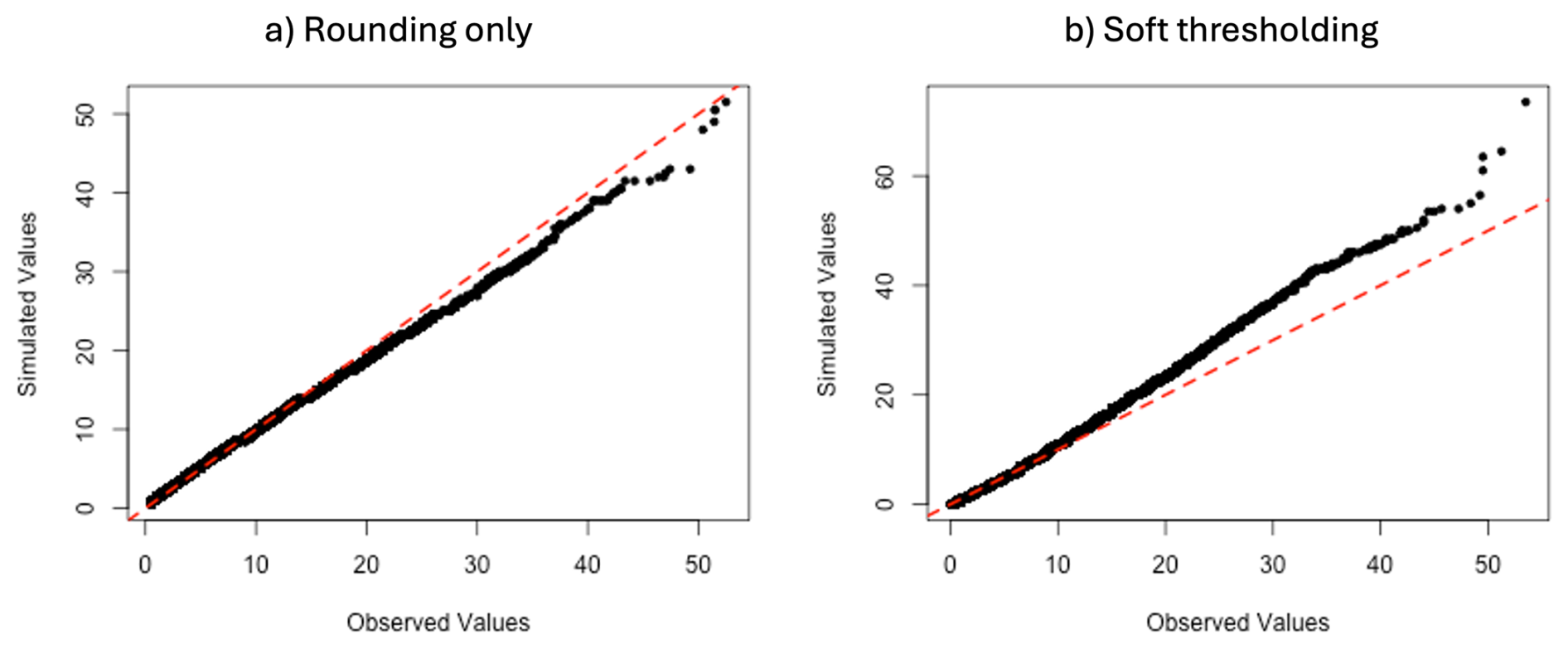
Figure A1 Quantile-quantile plots comparing the distributions of rounded samples from a Γ(5,1) distribution with those from gamma distributions fitted to them using maximum likelihood estimation. Panel (a) uses rounding only (estimated parameters: 5.244, 0.888); panel (b) uses soft thresholding (estimated parameters: 4.778, 1.212).

Soft thresholding: round all observations to the nearest 0.5, remove all values rounded to zero, and subtract 0.49 so that the smallest remaining value is 0.01.

Figure A1 shows the results. There are substantial mismatches between the upper tails of the “original” and “fitted” distributions under both rounding strategies, although in different directions. The reason is presumably that the shape parameter of a gamma distribution is strongly linked to the behaviour of its density in the lower tail where, by definition, rounding will substantially change the shape of the data distribution and where there are often many observations. This leads to biased estimates of the shape parameter when fitting the distribution, which has a knock-on effect in the upper tail where fewer observations are available to constrain the model fit.

Different ways are available to address this problem. In the work above we decide to work with data at recording resolution and account for changes in measurement accuracy using indicators as covariates within the model. As an alternative we note that estimation using the continuous ranked probability score (Gneiting and Raftery, 2007) leads to the correct upper tail behaviour, no matter the rounding strategy in the synthetic examples studied (not shown). This is in line with other literature reporting higher robustness of CRPS-based estimation (e.g. Gebetsberger et al., 2018) compared to that based on log-likelihoods. This should be explored further in future work.

Appendix B: Resampling approach for the WIC

The WIC requires that the resampled datasets {y^∗} can be regarded as drawn from the same distribution as the observations y. In simple settings, this is achieved by sampling from the observations with replacement – appealing to the standard bootstrap argument that the empirical distribution of a large number of observations will be close to the underlying data-generating distribution. For multisite precipitation, however, more care is needed to mimic sampling from the “real” data-generating process, which involves (i) dependence on covariates; (ii) residual inter-site dependence; and (iii) observations that are missing because only a subset of stations is reporting on any given day.

To account for dependence on covariates and residual inter-site dependence, the resampling is done by selecting full days, with replacement, from the period covered by the observations y. For each sampled day, all available precipitation values are added to the resampled dataset together with the corresponding covariates (including lagged precipitation values – which are added as covariates, rather than as additional rows in the dataset). However, this needs to be done in such a way that each resampled dataset has both the same number of days' data and the same number of individual observations as the original. Furthermore, if model selection is required for the combined occurrence/intensity model, then the same criteria should apply to the subset of resampled data containing only non-zero precipitation values.

To meet all of these requirements in the presence of many missing observations, we use stratified sampling in which days are split into groups (“strata”) containing the same number of non-missing observations and the same number of wet sites: days are then sampled from each stratum with replacement, such that the final resampled dataset contains the same number of days in each stratum as the original. This strategy requires that each stratum contains enough days to allow the creation of a large number of possible samples: this is the case for the dataset considered here.

With one exception, this resampling strategy allows model comparisons for the intensities and occurrence component of the integrated model separately. The exception relates to comparisons of occurrence models with and without an intercept, because all resampled datasets have the same total number of observations and the same number of wet days. Such comparisons are rarely of substantive interest however.

Appendix C: Estimation of inter-site dependence structure

When simulating multisite precipitation sequences, inter-site dependence is controlled via the correlation matrix Σ of multivariate standard Gaussian random variates, that are subsequently transformed using Eq. (10) to yield simulated precipitation. As described in Sect. 3.4, the elements of Σ are estimated separately for each pair of sites using maximum likelihood. Here we set out the calculations required to evaluate the required log-likelihood function, which must then be optimised numerically.

Suppose that for a given pair of sites, the available data consist of T pairs of observations $(y_{\mathrm{11}},y_{\mathrm{21}}),\mathrm{\dots },(y_{\mathrm{1}T},y_{\mathrm{2}T})$. If both sites are always wet, the inverse of Eq. (10) yields a corresponding set of pairs $(q_{\mathrm{11}},q_{\mathrm{21}}),\mathrm{\dots },(q_{\mathrm{1}T},q_{\mathrm{2}T})$ where $q_{\text{st}}={\mathrm{\Phi }}^{-\mathrm{1}}\left[{\mathit{\pi }}_{\text{st}}{F}_{\text{st}}\right(y_{\text{st}})+(\mathrm{1}-{\mathit{\pi }}_{\text{st}}\left)\right]$. When y_st=0, however, the corresponding value of q_st is not known exactly: all that is known is that $q_{\text{st}}\le {\mathrm{\Phi }}^{-\mathrm{1}}(\mathrm{1}-{\mathit{\pi }}_{\text{st}})$.

Under the proposed dependence model, the pairs {(q_1t,q_2t)} are all realisations of a bivariate normal random variable Q say, with mean vector 0 and covariance matrix $\left(\begin{array}{cc}\mathrm{1}& \mathit{\rho }\\ \mathit{\rho }& \mathrm{1}\end{array}\right)$ where ρ is the pairwise correlation to be estimated. Moreover, these realisations can be considered as independent if the marginal occurrence and intensity models contain an adequate representation of temporal dependence: see Chandler et al. (2007) for more discussion of this point. The log-likelihood for ρ is thus a sum of contributions from each of the T pairs, as follows:

Both sites wet: the contribution is the log of the bivariate normal density for (q_1t,q_2t).

Site 1 wet, site 2 dry: in this case, q_1t is known exactly but q_2t is known only to be less than ${\mathrm{\Phi }}^{-\mathrm{1}}(\mathrm{1}-{\mathit{\pi }}_{\mathrm{2}t})$. The log-likelihood contribution is obtained by factorising the joint density of Q as f₁(q_1t)f₂(q_2t|q_1t), in an obvious notation. Under the proposed model, the marginal distribution of Q_1t is standard normal; while the conditional distribution of Q_2t given Q_1t=q_1t is normal with mean ρq_1t and variance 1−ρ² (this is a standard result for the bivariate normal distribution). The log-likelihood contribution is thus

$$\log \mathit{\varphi }\left(q_{\mathrm{1}t}\right)+\log \mathrm{\Phi }\left({\displaystyle \frac{{\mathrm{\Phi }}^{-\mathrm{1}}(\mathrm{1}-{\mathit{\pi }}_{\mathrm{2}t})-\mathit{\rho }{q}_{\mathrm{1}t}}{\sqrt{\mathrm{1}-{\mathit{\rho }}^{\mathrm{2}}}}}\right),$$

where ϕ(⋅) and Φ(⋅) are, respectively the density and distribution function of the standard normal distribution. The first term does not involve ρ and can be dropped from the calculations.

Site 1 dry, site 2 wet: the contribution is analogous to that above, replacing q_1t and π_2t with q_2t and π_1t, respectively.

Both sites dry: here the contribution is $\log P(Q_{\mathrm{1}t}\le {\mathrm{\Phi }}^{-\mathrm{1}}(\mathrm{1}-{\mathit{\pi }}_{\mathrm{1}t}),Q_{\mathrm{2}t}\le {\mathrm{\Phi }}^{-\mathrm{1}}(\mathrm{1}-{\mathit{\pi }}_{\mathrm{2}t}\left)\right)$. For ρ≠0 this must be evaluated numerically: we use the mvtnorm package for this (Genz and Bretz, 2009).

If required, the likelihood of the latent correlation matrix can also be derived in the general case of S sites, using standard results for the density of a censored normal random variable (Hoffman and Johnson, 2011). Assume without loss of generality that among the S stations, stations $i=\mathrm{1},\mathrm{\dots },r$ design the dry and $r+\mathrm{1},\mathrm{\dots },S$ the wet stations, then the log-likelihood contribution of one day Y_t:=(Y_1t…Y_St)^T is proportional to:

$$\begin{array}{}\text{(C1)}& {\displaystyle }\log L\left(\mathbf{\Sigma }\right|{\mathit{Y}}_t)\propto \log {\mathit{\varphi }}_{\mathrm{\Sigma }}(q_{(r+\mathrm{1})t},\mathrm{\dots },q_{\text{St}})\text{(C2)}& {\displaystyle }\begin{array}{rl}& +\log {\mathbf{\Phi }}_{\mathrm{\Sigma }}\\ & \left({\mathrm{\Phi }}^{-\mathrm{1}}(\mathrm{1}-{\mathit{\pi }}_{\mathrm{1}t}),\mathrm{\dots },{\mathrm{\Phi }}^{-\mathrm{1}}(\mathrm{1}-{\mathit{\pi }}_{rt})|q_{(r+\mathrm{1})t}\mathrm{\dots },q_{\text{St}}\right).\end{array}\end{array}$$

Here $q_{(r+\mathrm{1})t},\mathrm{\dots },q_{\text{St}}$ can be calculated as $q_{\text{st}}={\mathrm{\Phi }}^{-\mathrm{1}}\left(F_{\text{st}}\right(Y_{\text{st}}\left)\right)$ and Φ_Σ,ϕ_Σ are the CDF and density of the latent standard multivariate Gaussian. This expression, however, can be cumbersome to compute due to the high cost of evaluating conditional normal distributions.

Appendix D: Model Building Strategy

We construct the occurrence and intensity models by sequentially adding covariates to the location parameter in the following order:

• 1.

  Base model. We begin with a model that includes lag-1 autocorrelation, data resolution, seasonality, and a spatial effect.

• 2.

  Model selection for autocorrelation, seasonal, and spatial effects. We refine the base model, selecting the most appropriate forms for representing seasonal and spatial variation as well as temporal dependence.

  • a.

    Spatial effect. For the parametric specification, we consider Legendre polynomials (up to degree three) and their interactions. For the semi-parametric specification, both spline-based (latitude–longitude) and Legendre polynomial representations are assessed, with the former ultimately being selected.

  • b.

    Seasonality. Competing formulations based on cyclic splines and parametric effects are compared for the semi-parametric models.

  • c.

    Autocorrelation. Beyond the lag-1 term, additional lags up to lag 3 are evaluated. For each lag, we assess:

    • the inclusion of main effects and their interactions with seasonal components,

    • whether to include lagged precipitation overall or indicator variables for lagged occurrences or both,

    • whether to employ spline-based or parametric formulations in the semi-parametric models, and

    • whether to include interactions between occurrence autocorrelation effects.

  • d.

    Additional interactions. We consider interactions between seasonal and spatial variation, and add site-specific effects such as altitude.

• 3.

  Large-scale atmospheric covariates. Finally, large-scale predictors and their interactions with seasonality are added in the following order:

  1. Temperature and possible interactions with seasonality.

  2. Dewpoint temperature and possible interactions with seasonality.

  3. Mean sea level pressure and possible interactions with seasonality.

  4. Wind speed, computed from the 10 m u- and v-wind components.

For the GAMLSS, we start with a full location model for intensity and build a model for the standard deviation by adding in order (1) seasonal variation, autocorrelation with resolution and their interactions; (2) Systematic spatial variation; (3) wind speed, temperature, dewpoint temperature, and mean sea level pressure in interaction with seasonality. In total around 40 models are compared for the parametric amounts model, and a similar number for the parametric occurrence as well as for both of the semi-parametric models.