the Creative Commons Attribution 4.0 License.
the Creative Commons Attribution 4.0 License.
 | 07 Oct 2020
Nonlinear time series models for the North Atlantic Oscillation
Thomas Önskog
Christian L. E. Franzke
Abdel Hannachi
The North Atlantic Oscillation (NAO) is the dominant mode of climate variability over the North Atlantic basin and has a significant impact on seasonal climate and surface weather conditions. This is the result of complex and nonlinear interactions between many spatio-temporal scales. Here, the authors study a number of linear and nonlinear models for a station-based time series of the daily winter NAO index. It is found that nonlinear autoregressive models, including both short and long lags, perform excellently in reproducing the characteristic statistical properties of the NAO, such as skewness and fat tails of the distribution, and the different timescales of the two phases. As a spin-off of the modelling procedure, we can deduce that the interannual dependence of the NAO mostly affects the positive phase, and that timescales of 1 to 3 weeks are more dominant for the negative phase. Furthermore, the statistical properties of the model make it useful for the generation of realistic climate noise.
- Article
(1230 KB) - Full-text XML
- BibTeX
- EndNote


The large-scale atmospheric flow has attracted the attention of climate scientists since the days of Gilbert Walker almost a century ago (see, e.g., Walker and Bliss, 1932, Rossby, 1940, Horel and Wallace, 1981, and the review of Hannachi et al., 2017, and the references therein). An important driving force behind this interest is the prospect of obtaining a better understanding of the different mechanisms involved and using this knowledge to predict the system on long lead times. Of particular interest is the challenge posed by the extratropical atmospheric variability, which exhibits both nonlinearity and considerable complexity.
The extratropical large-scale circulation can be described by a number of interacting teleconnection patterns, including the North Atlantic Oscillation (NAO) and the Pacific North America (PNA) pattern; see e.g. Wallace and Gutzler (1981), Hannachi et al. (2017) and Feldstein and Franzke (2017). These teleconnections are characterized by typically large spatial scales and low-frequency variability (timescales of more than 10 d; Feldstein, 2000, 2002, 2003; Franzke and Feldstein, 2005), which provides the potential for longer term predictability compared, for example, to synoptic scales.
Being one of the main teleconnection patterns of the Northern Hemisphere (NH), the NAO controls much of the atmospheric variability, particularly over the North Atlantic region, the Mediterranean and the Eurasian continent. It also interacts with other teleconnections, such as the PNA and the El-Niño–Southern Oscillation (ENSO), to produce remote responses. The NAO is known to have a direct, strong impact on surface weather and climate through changes in the atmospheric mass and shifts of the jet stream. It varies on a wide range of timescales, ranging from days to decades and longer (Woollings et al., 2014, 2015). Descriptions of the physical characteristics of the NAO can be found in Benedict et al. (2004), Franzke et al. (2004), Stendel et al. (2016), Hannachi and Stendel (2016) and the references therein.
Several meteorological centres issue regular forecasts of the NAO for various purposes (e.g. NOAA CPC, https://www.cpc.ncep.noaa.gov/products/precip/CWlink/pna/nao_index_ensm.shtml, last access: 5 October 2020). These forecasts are based on dynamical numerical weather prediction (NWP) models. Probabilistic or statistical models are also used to issue such forecasts on short and extended lead times. Statistical models have the advantage of being much simpler than their dynamical analogues, but this advantage comes at the expense of neglecting some interactions with other processes.
The NAO has a number of characteristic features. Its probability density function (PDF) is non-Gaussian, both in the bulk and in both tails of the distribution. Furthermore, the NAO has non-zero autocorrelation for short and long lags (see, e.g., Önskog et al., 2018). A good forecasting model for the NAO should, in principle, be able to reproduce these main properties. The non-Gaussianity implies, in particular, that linear models such as autoregressive (AR) models cannot reproduce the main features. Note, however, that linear models with non-Gaussian noise can of course produce non-Gaussianity (Franzke 2017; Önskog et al., 2018). The NAO is a nonlinear phenomenon and is related to synoptic Rossby wave-breaking (Benedict et al., 2004; Franzke et al., 2004) and regime behaviour (Hannachi et al., 2017). Based on this observation, it is reasonable to expect that nonlinear probabilistic models can be better suited to fit the NAO time series and be able to reproduce the properties mentioned above.
In a previous article (Önskog et al., 2018), we studied the properties of the time series of the daily NAO index, in particular the station-based time series published by Cropper et al. (2015), and found that the distribution of the NAO index has clear non-Gaussian features and long-range dependence (Franzke et al., 2020). An autoregressive model with non-standardized t-distributed noise, taking the values of the index during the last three days into account (AR), provided a good model for the daily NAO index on timescales of up to 2 weeks. By investigating forecasts of the future distribution of the NAO (considering both the expected value and quantiles), we found that some, but not all, properties were well described by the model. Features that the model was unable to replicate included the long-range dependence on timescales of the order of 20 d or more, the different timescales of the positive and negative phases of the NAO and the fact that the negative tail of the NAO distribution is fatter than the positive tail. In this article, we study nonlinear time series models and derive models that reproduce all these features of the daily NAO index. In addition to considering other classes of models compared to our previous article (Önskog et al., 2018), we also develop the test statistics used to compare and evaluate the models further.
Our aim here is to develop a statistical NAO model with which we will be able to identify important dynamical processes controlling the NAO. In order to make progress towards this aim, we here address the following specific research questions:
- i.
What are the nonlinearities and state-dependencies of the NAO distribution?
- ii.
Is there a nonlinear time series model which reproduces the properties of the NAO distribution?
- iii.
Does the inclusion of long lags on seasonal and interannual timescale improve a nonlinear model for the NAO?
Addressing these important research questions can help us to understand relevant physical processes controlling the NAO and, therefore, provide guidelines on which important physical processes to include in a statistical NAO model.
Our article is organized as follows. First, in Sect. 2, we shortly describe the time series of the winter NAO used in the article. Next, in Sect. 3, we investigate the statistical properties of this time series and describe some of the analyses that we carry out to evaluate the performance of the models that we propose. In Sect. 3.1, we briefly review the results on linear models obtained in Önskog et al. (2018) and also provide the rationale behind the model improvement. Section 4 defines four different nonlinear models for the NAO, including self-excited threshold AR models and state-dependent nonlinear models and models with nonlinear noise. Section 5 discusses the simulation of climate noise using the models derived, and a concluding discussion is presented in the final section.
In this study, we are using the daily time series of the NAO index published by Cropper et al. (2015). The index is calculated from actual sea level pressure (SLP) observations on Iceland and the Azores, but reanalysis data have been used to fill in the gaps (1888–1905, 1940–1941 and on 145 other occasional days) in the observations. These station-based data are freely available (https://zenodo.org/record/9979#.V_9RG037X4i, last access: 14 March 2019). In the generation of the time series, the seasonality was removed by applying a tension spline method in which a daily annual cycle (of mean SLP and the SLP standard deviation) was interpolated from monthly values and forced so that the average of the daily values of the curve for each month was equal to the monthly means. For details regarding the generation of the time series, we refer to the original source (Cropper et al., 2015).
We have restricted the present study to the winter season, which we here define as starting on 1 December and ending on 28 February (excluding 29 February for all leap years). The study is based on data for 142 consecutive winters from 1872/1873 to 2013/2014. We have chosen the 71 winters for which the month of December falls on an odd year (1873/1874, 1875/1876 and so on) as our training data for fitting of the models. The remaining 71 winters (1872/1873, 1874/1875 and so on) constitute our testing data used for validation of the models. Both training and testing data consist of 6390 data points each. We have chosen to spread the training and testing data evenly during the time period to reduce the effect of any non-stationarity in the data. Note that some of the nonlinear models studied in Sect. 4 below incorporate values of the NAO index during seasons other than the winter and during the period 1850–1871 as input.
The analyses of the models that we propose for the NAO will focus on the extent to which the models capture the distribution, autocorrelation and timescale of the NAO. The ability of the models to reproduce the distribution of the NAO will be visualized by means of density plots and Q–Q plots but also quantified in terms of the Kullback–Leibler divergence (Kullback, 1959; Kullback and Leibler, 1951; Cover and Thomas, 2006; Lacasa et al., 2012; Kowalski et al., 2011). The symmetrized Kullback–Leibler divergence (KLD) between two probability densities P,Q is defined as follows:
and similarly for DKL(Q|P). The KLD is non-negative for all choices of P,Q and provides a measure of the difference between two distributions. Note that . We will use the KLD as a measure of the distance between the empirical distribution of the NAO and the distributions simulated from the models proposed in this article. In this setting, both P and Q are discrete and are used to calculate the KLD between two discrete distributions, and we have used the default density kernel in R to obtain corresponding smooth probability densities and then the KLD function in R to calculate the KLD.
It should be noted that the comparisons based on KLD that we carry out are somewhat flawed by the fact that the simulated distributions are not fixed but influenced by statistical simulation error. However, in this study each simulated distribution is based on almost 1.3×10⁷ values, and for different realizations of the same model, the KLD between the empirical and the simulated distributions varies by an amount of the order of 10−4, which is negligible compared to the variation between different models. Furthermore, if we let P and Q be the empirical probability density of the training and testing data, respectively, we obtain . We do not expect the KLD between the NAO distribution simulated by any of the models proposed and the empirical NAO distribution for the testing data to fall much below this bound, but we note that slightly smaller values could occur, either due to statistical error or due to the distribution predicted by the model being, by chance, closer to the distribution of the testing data than to the distribution of the data it was trained on.
It is well known that the NAO distribution is non-Gaussian in the sense that both the skewness and excess kurtosis of its distribution are non-zero. Moreover, the values of higher moments and, hence, the size of the departure from normality, tend to depend on the current state of the NAO. In Fig. 1, we have plotted the values of the sample standard deviation, skewness and excess kurtosis as a function of the sample mean for each of the 71 winters in the testing data. We can see that the relations between higher moments and the first moment are close to linear, and Fig. 1 includes point estimates and confidence intervals for the intercept and the slope of the corresponding linear regression lines. The signs of the intercept and slope are significant for all three higher moments (see also the left plot in Fig. 2). In the coming sections, we will investigate how well the proposed models reproduce these linear relations.
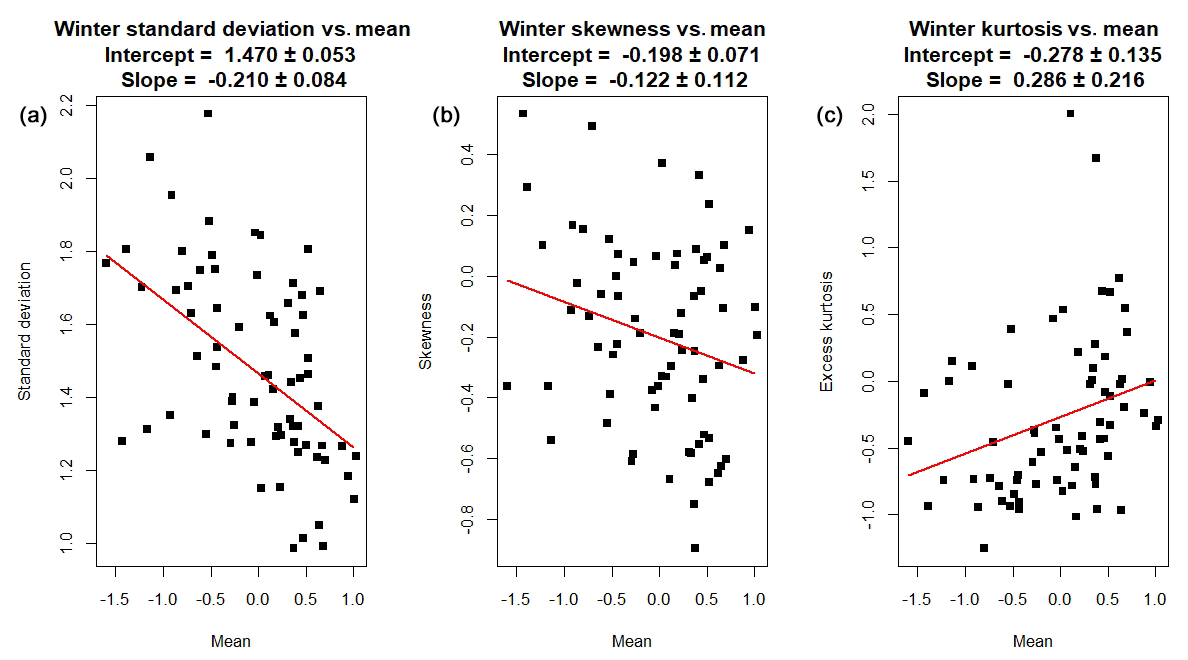
Figure 1Relation between higher moments of the daily North Atlantic Oscillation (NAO) winter index and the sample mean for 71 winters. The plots show the sample standard deviation (a), skewness (b) and excess kurtosis (c) as a function of the sample mean. The red lines are fitted regression lines. Point estimates and 95 % confidence intervals for the intercepts and slopes of these lines are given above each plot.
A simple measure for the persistence of NAO events is provided by the sample autocorrelation function (ACF). Figure 3 contains plots of the sample ACF for six choices of lags as a function of the sample mean for each of the 71 winters in the testing data. The sample ACF clearly decreases with increasing lag, but there is also a clear dependence on the sample mean, especially for lags up to 1 week and for lags of the order of 1 month. This can be interpreted as the negative state of the NAO being more persistent than the positive state, and also that the negative state has a negative autocorrelation for timescales around 1 month. The negative phase being more persistent than the positive phase is consistent with the dynamics of the NAO in that the negative phase corresponds to anticyclonic circulation, which is typically more persistent than cyclonic circulation corresponding to the positive NAO phase. In the right plot of Fig. 2 we have summarized the signs of confidence intervals of the intercept and slope of regressions of the sample ACF versus the winter mean for lags up to 45 d. In the coming sections, we will investigate how well the proposed models reproduce the sample ACF and its dependence on the winter mean.
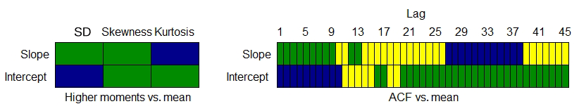
Figure 2Overview of the relations between higher moments and sample autocorrelation function (ACF) of the daily NAO winter index on one hand and the sample mean for 71 winters on the other hand. As described in the captions of Figs. 1 and 3, we have performed ordinary linear regressions and calculated 95 % confidence intervals for the intercepts and slopes of the regression lines. If a confidence interval is strictly positive, the corresponding field in the plot is blue, if a confidence interval is strictly negative, the corresponding field in the plot is green and if a confidence interval contains zero, the corresponding field in the plot is yellow.

Figure 3Relation between sample ACF of the daily NAO winter index and the sample mean for 71 winters. The plots show the sample ACF for lags 1, 8, 15, 22, 29, and 36, respectively. The red lines are fitted regression lines. Point estimates and 95 % confidence intervals for the intercepts and slopes of these lines are given above each plot.
3.1 Autoregressive models
In a previous study (Önskog et al., 2018), we found that an autoregressive (AR) model of order 3 with non-standardized t-distributed noise reproduces the distribution of the daily index of the NAO to some extent. Figure 4a–c compare the distribution of the daily winter NAO index to that of simulated values of the NAO index based on the AR model. We see that the AR model is unable to reproduce the skewness and tail behaviour of the NAO distribution. To quantify this, we note that the KLD between the probability densities of the testing data and the simulated AR model data is , which is 1 order of magnitude larger than the KLD between the training and testing data.
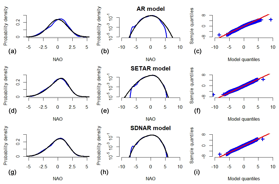
Figure 4(a–c) Properties of the autoregressive (AR), (d–f) self-exciting threshold autoregressive models (SETAR) and (g–i) state-dependent nonlinear autoregressive models (SDNAR) models for the daily NAO winter index. The plots in the left and middle columns show the probability density function (PDF) of the daily NAO winter index (blue) compared to the PDF of simulated values (black) in standard scale (a, d, g) and logarithmic scale (b, e, h). Panels (c), (f) and (i) show Q–Q plots of the daily NAO winter index compared to the simulated index.
Figure 5a displays the extent to which the AR model is able to reproduce the higher moments of the NAO and the linear dependences between the higher moments and the winter means. It is found that the model reproduces neither the average values nor the dependence on the winter means of higher moments. Figure 5b shows the ability of the AR model to reproduce the sample ACF of the NAO index and, in particular, the dependence between sample ACF and the winter means. The AR model reproduces the average value of the sample ACF very well, but it is unable to reproduce its dependence on the winter means.
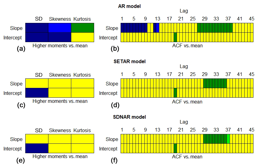
Figure 5Plot of the ability of the AR (a–b), SETAR (c–d) and SDNAR (e–f) models to reproduce the higher moments and sample ACF of the daily NAO winter index. The results are based on simulations of 142 000 winters, where the November data preceding each of the 71 winters in the testing data are used as initial values for simulations of 2000 winters. For the 142 000 winters, we have calculated the first four sample moments and sample ACF for lags 1–45 and performed linear regressions using ordinary least squares for all variables, with the sample mean as the explaining variable. Panels (a, c and e) show results for the regression intercept and slope for standard deviation, skewness and excess kurtosis, and panels (b, d and f) show the results for sample ACF for lags 1–45. The colours in the plots indicate the relation between the 95 % confidence intervals for the intercept or slope, based on simulations and the 95 % confidence interval of the corresponding regression parameter for the testing data. A confidence interval based on simulations can, in relation to the corresponding one based on observations, be strictly smaller (dark green), partly overlap but contain values smaller than the minimum of the interval based on observations (light green), overlap entirely (yellow), partly overlap but contain values larger than the maximum of the interval based on observations (light blue) or be strictly larger (dark blue), respectively.
We have also investigated the timescales of the two phases of the NAO. Following the procedure in Woollings et al. (2010), we first introduce two thresholds at ±1.64, which are approximately equal to plus and minus 1 standard deviation of the NAO index, to identify positive and negative NAO events. Then, for each of these events, we counted the number of subsequent days that were of the same phase. The data were then sorted to give a total of the number of events that lasted at least n days. Figure 6a shows the durations for the NAO index compared to the durations obtained by an AR model for the NAO index, and, as seen, the AR model is unable to differentiate between the timescales of the two phases.
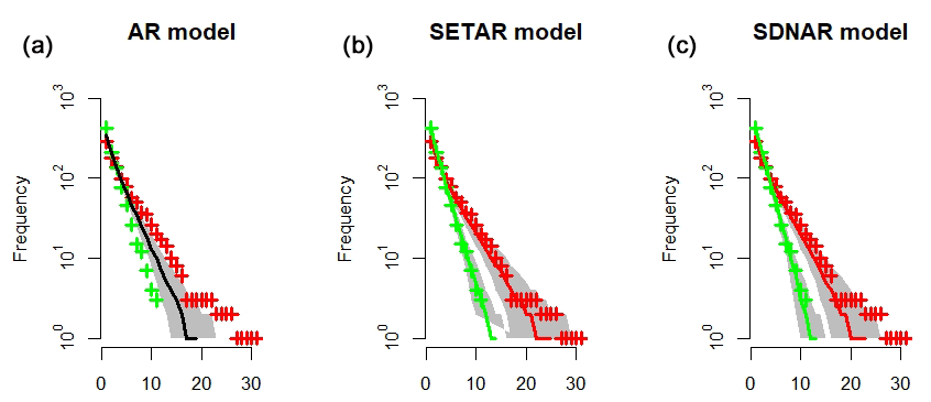
Figure 6Durations of the positive and negative phase of the NAO index as compared to durations derived from the AR (a), SETAR (b) and SDNAR (c) models. The plots show the absolute frequency of positive (green crosses) and negative (red crosses) phase events of the winter NAO index persisting more than a particular number of days. These frequencies are compared to those computed by the models for which the median (green and red lines, respectively) and 5 %–95 % range (grey regions) of 1000 realizations are displayed. For the AR models, the green and red lines overlap and are replaced by a black line.
3.2 Testing the hypothesis that the NAO is described by an AR model
It is unlikely that the skewness and different timescales of the two phases of the NAO can be reproduced by a linear autoregressive model, as such models stipulate the same probabilistic behaviour regardless of the current state of the NAO. To validate this conjecture, we conduct a statistical test on the hypothesis that all 142 winters in the data set can be successfully modelled by the same AR model. To this end, we have fitted AR models for all 142 winters separately using the Yule–Walker equations, first removing the mean of the particular winter. Let denote the three parameters in the AR model fitted to the NAO index for the ith winter in the data set. We saw in Fig. 3 that the lag 1 autocorrelation is slightly higher for winters when the negative phase is dominant. This is in agreement with the observation that negative NAO events persist longer than positive ones, and the same relationship holds between the first AR model parameters, , and the mean NAO index during the ith winter.
Under the null hypothesis that all winters are described by the same AR model with fixed, unknown parameters and standard deviation σ for the noise, it is well known (see e.g. Brockwell and Davis, 1991) that is approximately normally distributed with mean ϕ and covariance matrix . Here, n is the length of each winter, and the matrix Γp is defined as for , where γ(h) is the autocovariance function at lag h. Moreover, letting and denote, respectively, sample estimates of Γp and γ(h) for the ith winter, the following test statistic:
is approximately chi-square distributed with three degrees of freedom. Under the null hypothesis for the correct value of ϕ, the values of the test statistic for the 142 winters are a sample from an approximate chi-squared distribution with three degrees of freedom. We use the Kolmogorov–Smirnov test to calculate the p value for the event that the values of the test statistic come from a chi-squared distribution with three degrees of freedom. Regardless of the choice of ϕ, the p value does not exceed 0.008. Thus, we can reject the hypothesis that all 142 winters are well described by the same AR model.
An analysis of the parameters of the 142 AR models for the various years shows that there is no significant autocorrelation in the parameters. As these parameters are related to the autocorrelation of the daily winter NAO index for the different years, the absence of significant autocorrelation in the parameters should be interpreted as a lack of interannual dependence between the perturbations of the sample ACF from its mean. Conclusively, any interannual dependence in the winter NAO is due to the dependence of the actual value on past states of the index and not due to a dependence in its autocorrelation function.
In this section, we consider a couple of classes of nonlinear time series models and investigate whether they provide a better fit of the daily winter NAO index than standard linear AR models.
4.1 Self-exciting threshold autoregressive models (SETAR)
We conclude from Figs. 1 and 3 that both the distribution and the autocorrelation structure of the daily winter NAO differ between the positive and the negative phase. This regime behaviour has previously been noted by Woollings et al. (2010), Franzke and Woollings (2011) and Franzke et al. (2011) for the North Atlantic sector. A natural way of constructing a model, taking this feature into account, is to use different AR models for the different phases of the daily winter NAO. Such a model is known as a self-exciting threshold autoregressive (SETAR) model and is natural to consider, given previous observations of the existence of two regimes for the NAO (Woollings et al., 2010). Let be a partition of the real line into k regions or regimes separated by the thresholds . A SETAR(p) model Yt is defined as follows:
for . Here, , for and , are real valued parameters, for some real numbers of σ(i) and , and I(x) is the indicator function taking the value one if x is true and zero otherwise (see e.g. De Gooijer, 2017).
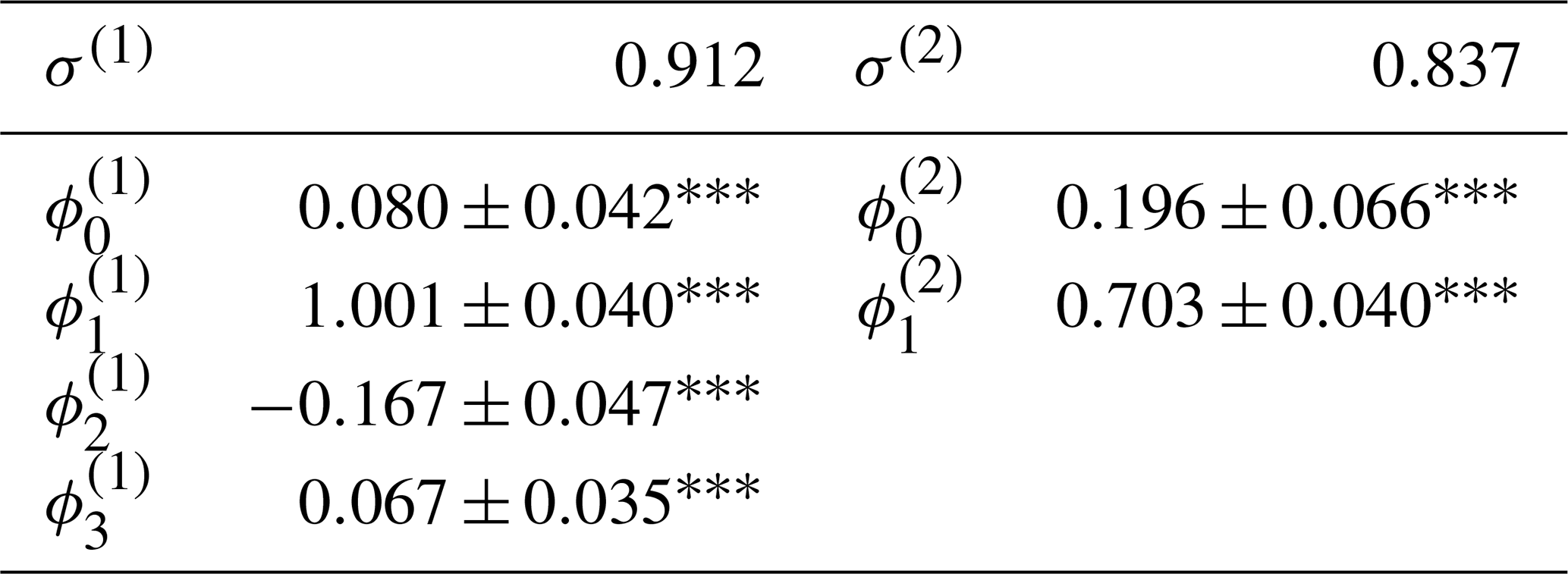
As the optimal order of AR models for the daily winter NAO index was found to be three in Önskog et al. (2018), we also use p=3 in the SETAR model for the daily winter NAO. Using a two-regime model with threshold r1=0.39, obtained from a grid search over the set of possible thresholds, the optimal parameters in the SETAR model are given in Table 1. The time series containing all winters is discontinuous between different years, so the process of fitting the SETAR model to the data requires some special care. First, we have categorized every day in the time series according to which regime Yt−1 belongs. For both regimes, we have registered the values of Yt−j and (note that on December 1–3 this requires knowledge of some autumn values of the NAO), and then we performed ordinary multiple linear regression of Yt on Yt−j for . The Bayesian information criterion (BIC) was used to determine which factors to include in the final model. Note that the lag 2 and lag 3 parameters, and , respectively, are not significant in the right (positive) regime. Note also that the lag 1 parameter is smaller in the right regime than in the left regime, and that this observation is consistent with the shorter timescale of the positive phase of the NAO.
Table 1Parameter estimates for the SETAR model for the daily winter NAO index. Here, and throughout the article, denotes parameters that are significant, with p value <0.001; denote parameters that are significant, with p value in the interval [0.001,0.01); and * denote parameters that are significant with p value in the interval [0.01,0.05).
The distributional properties of the SETAR model are shown in the second row of Fig. 4. The SETAR model reproduces the distribution of the daily NAO index well, with the exception of both tails of the distribution which the model exaggerates. The KLD between the probability densities of the testing data and the simulated SETAR model data are , which is just 10 % larger than the KLD between the training and testing data. As Fig. 5c–d show, the model reproduces the dependence of the second, third and fourth order moments on the winter mean. The average of the sample ACF is well approximated by the SETAR model for all lags, but the positive correlation between the sample ACF of lags of the order of 4–5 weeks and the winter mean is missed by the model. As seen in Fig. 6b, the SETAR model reproduces the durations of both the negative and positive phases of the NAO very well.
4.2 State-dependent nonlinear autoregressive models (SDNAR)
Instead of assuming distinct regimes for the different phases of the NAO, we may assume that the parameters of an AR model depend on the present state of the NAO. If we assume parameters of an AR(p) model to be polynomials of, at most, second order, we obtain a state-dependent AR(p) model with cubic power, here abbreviated as SDNAR(p). An SDNAR(p) model Yt is defined as follows:
for . Here, ϕ0 and , for and , are real valued parameters, and εt denotes white noise that is .
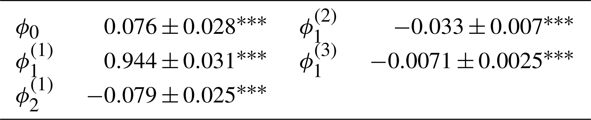
As for the AR and SETAR models, we use p=3 for the SDNAR model, but as the lag 3 terms turn out to be insignificant in this setting, our final model turns out to be an SDNAR(2) model. To fit the SDNAR model to the data, we have registered, for every day Yt in the time series, the values of (as for the SETAR model, this requires knowledge of some autumn values of the NAO) and performed ordinary multiple linear regression of Yt on , for . The BIC was used to determine which terms have a significant impact. The result is given in Table 2. As seen, the quadratic and cubic lag 1 terms, and , respectively, are significantly different from zero. Note also that the error is normally distributed with standard deviation 0.879.
Table 2Parameter estimates for an SDNAR model for the daily winter NAO index.
The distributional properties of the SDNAR model are shown in the lower row of Fig. 4. The SDNAR model reproduces the distribution of the daily NAO index even better than the SETAR model and the KLD between the probability densities of the testing data and the simulated SDNAR model data are , which is actually smaller than the KLD between the training and testing data. As Fig. 5e–f show, the SDNAR model reproduces the higher moments and sample ACF to the same extent as the SETAR model. Moreover, as Fig. 6b–c show, the SDNAR and SETAR show similar, excellent, skill in reproducing the durations of both the negative and the positive phases of the NAO. All subsequent models considered in this article show the same excellent skill in reproducing the durations of the two NAO phases, and the duration plots for these models have hence been omitted.
4.3 Nonlinear autoregressive models with longer lags (extended SETAR and SDNAR)
From Figs. 4 and 5, it is seen that the SETAR and SDNAR models do not perfectly reproduce all properties of the PDF and sample ACF of the daily winter NAO. As an attempt to construct a model that gives a better description of the sample ACF, we have constructed an extended linear regression model, including a number of additional terms with longer lags, and we reduced the model complexity stepwise, using the BIC as parameter selection criterion until only the significant parameters remain. In addition to the variables used in the SDNAR model, the initial regression model included the factors , the mean of , the mean of , the mean of , the mean of the preceding autumn, summer and spring, respectively and, lastly, the mean of each of the last 16 winters. Note that some of these variables include NAO index values for seasons other than the winter.
The final model, which we refer to as the extended SDNAR (ESDNAR) model, is very similar to the SDNAR model. The variables included in the model are the same, except that the ESDNAR model includes an additional Yt−7 term. Moreover, the parameter values differ by less than 0.004, and as a consequence, the performance of the two models is very similar. For example, the KLD is for the ESDNAR model – just as for the SDNAR model. The plots of the distribution of the ESDNAR model have been omitted, but Fig. 7a–b show the higher moments and sample ACF of the ESDNAR model. The results for the ESDNAR model are very similar to those of the SDNAR model but, in general, slightly better.
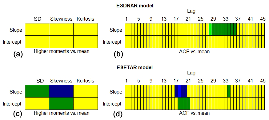
Figure 7Plots of the ability of the extended SDNAR (ESDNAR) (a, b) and extended SETAR (ESETAR) (c, d) models to reproduce the higher moments and sample ACF of the daily NAO winter index. The plots are generated in the same way as the plots in Fig. 5.
In a similar fashion, the SETAR model can be supplemented by additional terms with longer lags. Using the thresholds and r2=0.82, approximately corresponding to minus and plus one half standard deviation, we find the significant parameters in the three regimes listed in Table 3 below. In the process of choosing parameters, we have used the BIC as a selection criterion to make sure that terms which do not give a significant contribution do not remain in the final model. The lag 1, lag 2 and lag 7 terms are significant in the left regime, as was the case also for the ESDNAR model, but also the mean of the NAO 15–21 d ago. In the middle regime, only the lag 1 and lag 2 terms are significant, and in the right regime the lag 1 term and the mean of the NAO seven winters ago are significant. Based on the significant terms in this extended SETAR model, which we from now on refer to as the ESETAR model, we can draw some interesting conclusions regarding the timescales of the different phases of the winter NAO. In the negative phase of the NAO, a lag 7 term and the mean 15–21 d prior to the present date gives a significant contribution to the model, but there are no significant inter-seasonal or interannual terms. Terms with lags of the order of 1–3 weeks for the negative phase come as no surprise, as we know from observations that there is an increased proportion in negative phase events of such lengths. In the positive phase of the NAO, a term for the seventh last winter is significant, showing that, except for the lag 1 term, there is only dependence on very long timescales (almost interdecadal). These results indicate that the interannual dependence of the NAO mostly affects the positive phase and that timescales of 1–3 weeks are most dominant for the negative phase. It should be noted, however, that the extended regression included 33 additional variables, and that the large amount of covariates increases the risk that one or more covariate is spuriously significant. The p values of the long lag variables included in the ESETAR model are 0.0029 and 0.0047, respectively, and the probability of obtaining such a low p value for at least one of the variables purely by chance when investigating 33 variables is of the order of 10 %–15 %.
Table 3Parameter estimates for an ESETAR model for the daily winter NAO index.
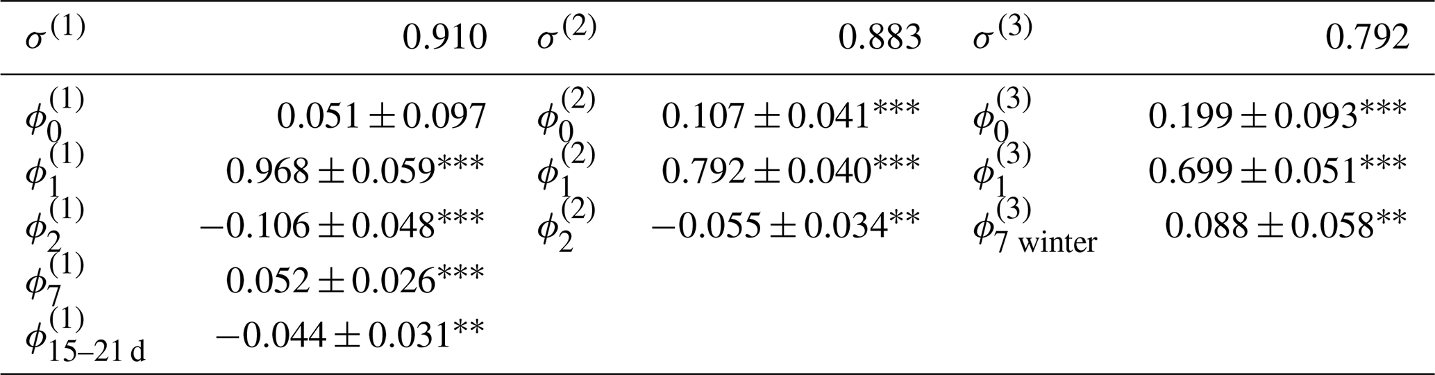
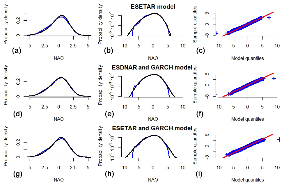
Figure 8a–c show the distributional properties of the ESETAR model. The ESETAR model is slightly worse than the SETAR model at reproducing the bulk of the distribution, and the KLD for the ESETAR model is , which is twice as much as for the SETAR model. Moreover, as seen in the lower row of Fig. 7, the higher moments are reproduced worse by the ESETAR model than the SETAR model. On the other hand, the ESETAR model gives a very good fit of the sample ACF, both in terms of intercept and slope, and in contrast to all previously considered models, it reproduces the positive correlation between the sample ACF of lags of the order of 4–5 weeks and the winter mean.
4.4 Models with nonlinear noise
Up to now we have assumed the noise in all models to be independent and identically normally distributed. A necessary condition for the independence of the elements of a time series is that the sample ACF of the squared entries in the series is close to zero, and this fact can be used as a test of independence. If a nonlinear model captures all the dependencies in the data, we expect the sample ACF of squared residuals of the model to be close to zero for all lags. But the lag 1 sample ACF of the squared residuals of all models investigated up to now is between 0.035 and 0.045, which is significantly larger than zero (at 5 % significance level, the values differing more than 0.025 from zero are significantly non-zero for time series of the length used here), whereas for larger lags the sample ACF is not significantly non-zero. This implies that large residuals in terms of absolute value are likely to be followed by residuals with large absolute value and vice versa, and that the error variance can be well modelled by an autoregressive model.
4.4.1 Generalized autoregressive conditional heteroskedasticity (GARCH) noise
The noise clustering described above is often successfully modelled by a generalized autoregressive conditional heteroskedasticity (GARCH) process (see e.g. De Gooijer, 2017). A GARCH(p,q) process {Zt} is defined as follows:
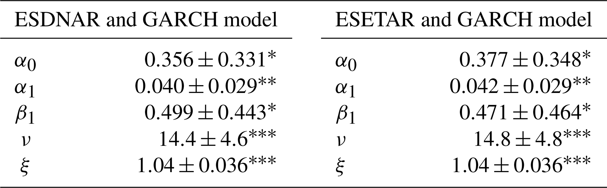
and et is independent and identically distributed noise. We fit the residuals of the nonlinear models to a GARCH(1,1) process, and based on the results in Önskog et al. (2018), we model {et} as an independent, skewed t-distributed time series with ν degrees of freedom and skew parameter ξ. For the ESDNAR and ESETAR models, the optimal choice of GARCH parameters are given in Table 5.
Considering now, instead of the residuals from the ESDNAR and ESETAR models, the standardized residuals obtained by dividing the residuals by , the non-zero lag 1 sample ACF of the squared residuals vanishes and this indicates independence of standardized residuals. An even better test for independence is the Brock, Dechert and Scheinkman (BDS) test (Brock et al., 1996), which we now shortly describe. Let , and then define the correlation integral with dimension m and distance ϵ as follows:
where is 1 if the supremum norm of is below ϵ and 0 otherwise. The correlation integral is a measure of the proportion that any pairs of m vectors ( and ) are within a certain distance ϵ. If the time series {Xt} is indeed independent and identically distributed (i.i.d.), then should exhibit no pattern in the m-dimensional space, so that . The BDS test is designed to check whether the sample counterparts of C(m,ϵ) and C(1,ϵ)m are sufficiently close. Often, this closeness is tested for a number of choices of the parameters m and ϵ.
Table 4GARCH parameter estimates for the noise in the extended models. Note: “ESDNAR and GARCH” denotes the ESDNAR model with GARCH noise, and “ESETAR and GARCH” denotes the ESETAR model with GARCH noise.
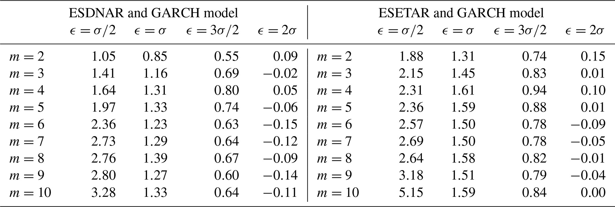
Applying the BDS test to the standardized residuals, we obtain the values shown in Table 5 below. Under the null hypothesis of independence of the standardized residuals, 95 % of the entries in Table 5 should be within ±1.96. We note an overrepresentation of values exceeding 1.96 for and large m, and this corresponds to too many events of subsequent small residuals.
Table 5BDS test results for the standardized residuals of the GARCH noise models. The test has been performed with parameter values and , where σ is the sample standard deviation of the residuals. Note: “ESDNAR and GARCH” denotes the ESDNAR model with GARCH noise, and “ESETAR and GARCH” denotes the ESETAR model with GARCH noise.
Although the application of GARCH noise in the model explains most of the dependence in the noise, it does not improve the fit of the distributional properties of the daily winter NAO index. The last two rows in Fig. 8 show that the models with GARCH noise exaggerate the tails of the NAO distribution more than the corresponding models with i.i.d. noise. Comparing the sample ACF of the models with GARCH noise in the first two rows of Fig. 9 with the results in Fig. 7, we note that the GARCH noise models perform very similar to the models with normally distributed noise.
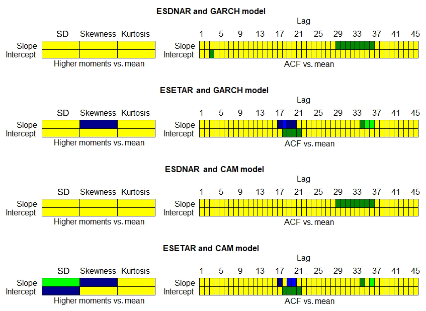
Figure 9Plots of the ability of the ESDNAR model with GARCH noise, denoted as ESDNAR and GARCH, (first row); the ESETAR model with GARCH noise, denoted as ESETAR and GARCH, (second row); ESDNAR and correlated additive and multiplicative (CAM) noise, denoted as EDSNAR and CAM, (third row); and the ESETAR model with CAM noise, denoted as ESETAR and CAM, (fourth row) models to reproduce the higher moments and sample ACF of the daily NAO winter index. The plots are generated in the same way as the plots in Fig. 5.
4.4.2 Correlated additive and multiplicative (CAM) noise
The application of GARCH noise in the models explains most dependence in the noise, but it does not improve the fit of the NAO distribution and does not give a clear improvement of the fit of the sample ACF. We therefore implement another type of noise which has previously been suggested in the literature (Sardeshmukh and Sura, 2009; Majda et al., 2009; Franzke, 2017), namely correlated additive and multiplicative (CAM) noise. We define a time series model Yt with CAM noise as follows:
where μ,σ2 are real valued constants, F is a (linear or nonlinear) function, which in our case is piecewise polynomial, σ1 is a positive constant and {ηt} is a sequence of independent, standard normally distributed random variables. Here can represent the right-hand sides of Eqs. (3) or (4) but with the noise removed. Note that the additive and multiplicative parts of the noise considered in Eq. (7) are perfectly correlated. This is a special case of the general definition of CAM noise in which the additive and multiplicative parts of the noise have the correlation coefficient . With CAM noise, the size of the noise depends linearly on the current state of the NAO. We note that this is consistent with the gradual decrease in the parameters σ(i) in the ESETAR model as i increases. The size of the noise on subsequent days is not directly dependent, as was the case for GARCH noise, but indirectly in the sense that days with negative phase (and larger noise) are more likely to be followed by days with negative phase (and larger noise) and vice versa. To implement CAM noise, we first determine from the training data using some of the methods described earlier in this article, and then we use the method of moments to estimate σ1 and σ2. To this end, we first define four different sample means as follows:
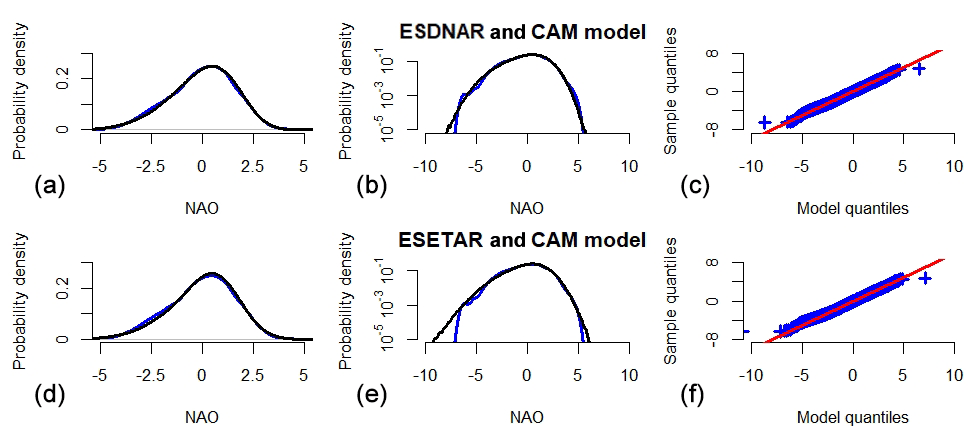
Figure 10Properties of the ESDNAR model with CAM noise (a, b, c), denoted as ESDNAR and CAM model, and the ESETAR model with CAM noise (d, e, f), denoted as ESETAR and CAM model, models for the daily NAO winter index. The plots are generated in the same way as the plots in Fig. 4.
These sample means are easily calculated given the choice and the training data. By the method of moments, we expand the expectations of and and obtain the following set of equations for the unknown parameters σ1 and σ2:
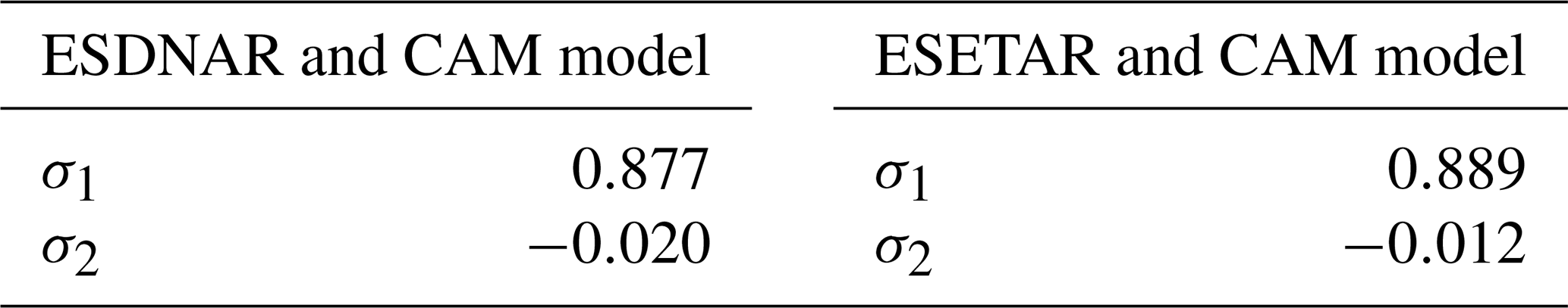
expressed in terms of the estimates of the sample means and d. Solving these equations for σ1,σ2 with corresponding to the ESDNAR and ESETAR models, respectively, we obtain the parameter estimates in Table 7 below. We note that the multiplicative part of the noise is quite weak, and that the sign of the multiplicative term is consistent with larger noise for the negative phase of the NAO.
Table 6CAM parameter estimates for the noise in the extended models. Note: “ESDNAR and CAM model” denotes the ESDNAR model with CAM noise, and “ESETAR and CAM model” denotes the ESETAR model with CAM noise.
Comparing Figs. 8 and 10, we see that the CAM noise gives a slightly better fit of the NAO distribution. As a comparison, the KLD is and for the ESDNAR and ESETAR models with CAM noise as compared to and for the ESDNAR and ESETAR models with GARCH noise. For the fit of the sample ACF, the GARCH and CAM noise models perform very similarly (see Fig. 9). But running the BDS test for the models with CAM noise (see Table 8 below), we see that the CAM noise is unable to remove the dependence in the noise as efficiently as the GARCH noise. To put the results into context, it should be mentioned that the values of the BDS test variable for the models with normally distributed noise are in general 0.2–0.4 higher than the values for the corresponding model with CAM noise. Hence, the CAM noise model reduces the dependence of the noise slightly, but not sufficiently.
Table 7BDS test results for the standardized residuals of the CAM noise models. The test has been performed with parameter values and , where σ is the sample standard deviation of the residuals. Note: “ESDNAR and CAM model” denotes the ESDNAR model with CAM noise, and “ESETAR and CAM model” denotes the ESETAR model with CAM noise.

The models investigated in this article only use present and past values of the NAO index to compute the future NAO index and not any other covariates. For this reason, the predictive skill of these models will be inferior to that of dynamical models taking many other variables than the NAO index itself into account. To give an example, comparing the forecast skill of one of the nonlinear statistical models proposed in this article to that of the dynamical forecast model issued by NOAA (ftp://ftp.cpc.ncep.noaa.gov/cwlinks/norm.daily.nao.ensf.z500.b14sep2001_current, last access: 17 May 2019), we see that the mean absolute error (MAE) of the 1 d forecast of the statistical model is similar to the MAE of the 6 d forecast of the NOAA model. However, in this context, we stress that the comparison between the dynamical and statistical models is flawed by the fact that the NAO index used by NOAA is based on reanalysis data which are differently normalized than the station-based data used in this article and, as a result, we cannot directly compare the results of the two classes of models. Moreover, the reanalysis data-based NAO index, being based on an empirical orthogonal function analysis, is much smoother than the station-based NAO index and this will affect the predictability of the two types of NAO indices.
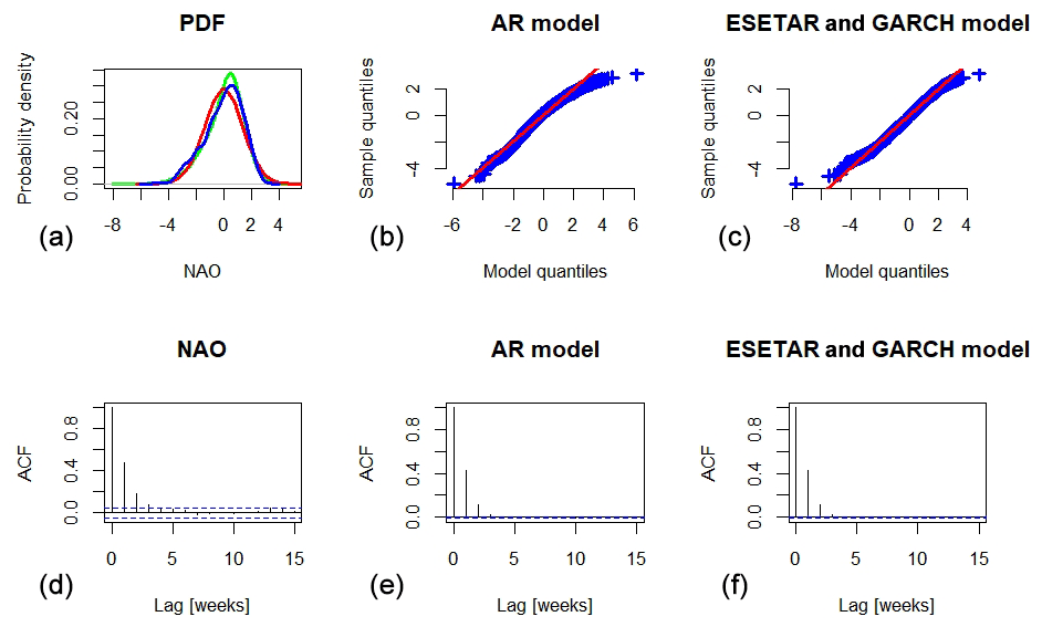
Figure 11Simulation of weekly means of the NAO. Panel (a) shows the PDF of weekly means of the observed daily NAO winter index (blue) compared to weekly means of simulated NAO index obtained by the AR model (red) and the ESETAR model with GARCH noise, denoted as “ESETAR and GARCH model”, (green), respectively. Panels (a–c) are Q–Q plots of the weekly means of the daily NAO winter index compared to the simulated indices. Panels (d–f) show the sample ACF of weekly means of the observed daily NAO winter index (d), the simulated index obtained by the AR model (e) and the simulated index obtained by the ESETAR model with GARCH noise (f). Confidence intervals with confidence level 95 % are indicated by dashed blue lines in the sample ACF plots.
We next investigate if simulations of the models proposed in this article generate surrogate time series which have the same properties as the daily winter NAO index on timescales other than days. To this end, we have simulated n=10 000 winters of daily NAO data with the AR and ESETAR model with GARCH noise, respectively. Although the ESDNAR model with GARCH noise generally reproduces the daily NAO index slightly better than the ESETAR model with GARCH noise, we have chosen to use the latter model here as it contains terms with longer lags, which could help capturing long-term relationships. To obtain starting values for each of the winters, we have run the models for 2 months. We have calculated weekly, monthly and winter means of the simulated NAO and compared these means to those of the observed NAO index in terms of PDF and sample ACF. Figure 11 shows that the ESETAR model with GARCH noise reproduces the distribution of weekly means of the daily winter NAO index slightly better than the AR model and that both models perform similarly with respect to the sample ACF. The models slightly underestimate the sample ACF, but the difference is not significant.
Figures 12 and 13 show that the sample ACF for the monthly means is significantly different from zero for lags of 1 and 4 months, with sample ACF values just above 0.1. For the winter means, the sample ACF is not significantly different from zero for any choice of lag. The lag 1 sample ACF for the monthly means is captured by both models, but not the lag 4 value. We note that the term corresponding to the mean of the winter of 7 years ago does not give rise to any significantly non-zero sample ACF, neither for the winter means nor for the monthly means, and this is reflected by the absence of non-zero sample ACF for the winter NAO for all interannual lags. The ESETAR model with GARCH noise provides a slightly better fit of the NAO PDF than the AR model. It is interesting to note that the distribution of the observed winter means almost appears to be bimodal, but this is probably an effect of too short a time series. A Kolmogorov–Smirnov test for normality has p value 0.21, so we cannot reject the hypothesis that the distribution of winter means is normal.
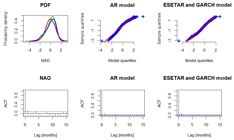
Figure 12Simulations of monthly means of the NAO. The plots are identical to Fig. 11, but with weekly means replaced by monthly means.

In this study we have shown that the NAO can be well described by nonlinear autoregressive models. Different models have different benefits and drawbacks, but in general the performances of the various nonlinear models are fairly similar. Putting all the analyses together, the time series model that provides the best description of the station-based daily winter NAO index is of polynomial form with GARCH-type noise. This model is able to reproduce the skewness and fat tails of the observed NAO index and the autocorrelation and timescales of the positive and negative phases of the NAO. The nonlinear and state-dependent NAO model gives some indication of dominant timescales for the NAO. Our model elucidated that the interannual variability mainly affects the positive phase of the NAO, while the negative phase is more affected by processes acting on timescales of 1–3 weeks. These findings are in agreement with the recent results of Caian et al. (2018), who analysed the interannual link between Arctic sea ice and the NAO using reanalysis data and climate model simulations. It was found, in particular, that anomalous Arctic sea ice, associated with a quasi-steady positive gradient of sea ice anomalies about coastal line, act to force precisely the positive NAO phase on interannual timescales.
Interestingly, the ESETAR model for the NAO index reveals significant association with slow timescales of the order of 7 years. A similar long-range behaviour for the NAO has previously been observed in several studies on the spectrum of the NAO, which found peaks of the NAO spectrum in the broad range of 7–10 years (e.g. Gámiz-Fortis et al., 2002; Wunsch 1999). This extended range dependence could be an imprint of the Hurst phenomenon (e.g. Franzke et al., 2020) and has been observed in various branches of natural sciences, such as hydrology (Mandelbrot and Wallis, 1968) and the atmospheric circulation (Franzke et al., 2015b). However, this long timescale did not show up in the sample ACF of the NAO time series, and it is unclear if this is due to the limited length of the data or that the dependence is not manifested in the sample ACF.
The better performance of the SDNAR model compared to the SETAR model might suggest that it is not possible to straightforwardly represent the nonlinearity by conditional linear models as was proposed by Horenko (2010), O'Kane et al. (2013), Franzke et al. (2015a) and Risbey et al. (2015). The idea, in these studies, is that the nonlinear behaviour of the atmospheric circulation can be captured by piecewise linear models. While models in these studies are not exactly similar to the SETAR class of models, they share the underlying idea.
The NAO is not an isolated and self-sustained phenomenon. It interacts with many other processes, including mainly the bottom boundary forcing. The sea surface temperature, for example, varies on a wide range of timescales, with the particular predominance of low frequencies, and can affect the NAO on those scales. Land surface and, in particular, sea ice interactions, can also affect NAO variability on those same scales. A comprehensive probabilistic model for the NAO that is able to provide a better long-term prediction should possibly include those processes as predictors, in addition to the nonlinear terms considered here. This is beyond the scope of this paper and is left for future research.
The station-based data for the daily NAO index are freely available online at https://doi.org/10.5281/zenodo.9979 (Cropper et al., 2014).
TÖ constructed the models, carried out the simulations and wrote Sects. 2–5 of the paper. CLEF and AH provided ideas, suggested improvements during the entire process of conducting the research and contributed to Sects. 2–5. All authors contributed to the writing of Sects. 1 and 6.
The authors declare that they have no conflict of interest.
We would like to thank Stephen Baxter and Jon Gottschalck at NOAA's Climate Prediction Center for kindly providing us with data about the NOAA forecasts. CLEF was partially supported by the Collaborative Research Centre (grant no. TRR 181) “Energy Transfer in Atmosphere and Ocean”, funded by the Deutsche Forschungsgemeinschaft (DFG – German Research Foundation) under project 274762653 (grant no. FR3515/3-1). Four anonymous reviewers provided constructive comments that helped improve the paper.
This research has been supported by the DFG, German Research Foundation (grant no. 274762653).
This paper was edited by Chris Forest and reviewed by four anonymous referees.
Benedict, J. J., Lee, S., and Feldstein, S. B.: Synoptic view of the North Atlantic oscillation, J. Atmos. Sci., 61, 121–144, 2004.
Brock, W. A., Dechert W. D., and Sheinkman J. A.: A test of independence based on the correlation dimension, Econom. Rev., 15, 197–235, 1996.
Brockwell, P. J. and Davis, R. A.: Time series: Theory and methods, second edition, Springer, New York, https://doi.org/10.1007/978-1-4419-0320-4, 1991.
Caian M., Koenigk, T., Döscher, R., and Devasthale, A.: An interannual link between Arctic sea-ice cover and the North Atlantic Oscillation, Clim. Dynam., 50, 423–441, 2018.
Cover, T. M. and Thomas, J. A.: Elements of information theory, 2nd Edn., John Wiley & Sons, Hoboken, New Jersey, https://doi.org/10.1002/047174882X, 2012.
Cropper, T., Hanna, E., Valente, M. A., and Jónsson, T.: A daily Azores-Iceland North Atlantic Oscillation index back to 1850, Geosci. Data J., 2, 12–24, 2015.
Cropper, T. E., Hanna, E., Valente, M. A., and Jónsson, T.: A daily Azores-Iceland North Atlantic Oscillation Index back to 1850, Zenodo, https://doi.org/10.5281/zenodo.9979, 2014.
De Gooijer, J.: Elements of nonlinear time series analysis and forecasting, 1st Edn., Springer International Publishing, https://doi.org/10.1007/978-3-319-43252-6, 2017.
Feldstein, S. B.: The timescale, power spectra, and climate noise properties of teleconnection patterns, J. Climate, 13, 4430–4440, 2000.
Feldstein, S. B.: Fundamental mechanisms of the growth and decay of the PNA teleconnection pattern, Q. J. Roy. Meteor. Soc., 128, 775–796, 2002.
Feldstein, S. B.: The dynamics of NAO teleconnection pattern growth and decay, Q. J. Roy. Meteor. Soc., 129, 901–924, 2003.
Feldstein, S. B. and Franzke, C.: Atmospheric teleconnection patterns in: Nonlinear and Stochastic Climate Dynamics, edited by: Franzke, C. L. E. and O'Kane, T. J., Cambridge University Press, Cambridge, UK, 54–104, 2017.
Franzke, C.: Extremes in dynamic-stochastic systems, Chaos, 27, 012101, https://doi.org/10.1063/1.4973541, 2017.
Franzke, C. and Feldstein, S. B.: The continuum and dynamics of Northern Hemisphere teleconnection patterns, J. Atmos. Sci., 62, 3250–3267, 2005.
Franzke, C. and Woollings, T.: On the Persistence and Predictability Properties of North Atlantic Climate Variability, J. Climate, 24, 466–472, 2011.
Franzke, C., Woollings, T., and Martius, O.: Persistent Circulation Regimes and Preferred Regime Transitions in the North Atlantic, J. Atmos. Sci., 68, 2809–2825, 2011.
Franzke, C., Lee, S., and Feldstein, S. B.: Is the North Atlantic Oscillation a breaking wave?, J. Atmos. Sci., 61, 145–160, 2004.
Franzke, C. L. E., O'Kane, T. J., Monselesan, D. P., Risbey, J. S., and Horenko, I.: Systematic attribution of observed Southern Hemisphere circulation trends to external forcing and internal variability, Nonlin. Processes Geophys., 22, 513–525, https://doi.org/10.5194/npg-22-513-2015, 2015.
Franzke, C., Osprey, S. M., Davini, P., and Watkins, N. W.: A dynamical systems explanation of the Hurst effect and atmospheric low-frequency variability, Sci. Rep., 5, 9068, 2015b.
Franzke, C., Barbosa, S., Blender, R., Fredriksen, H. B., Laepple, T., Lambert, F., Nilsen, T., Rypdal, K., Rypdal, M., Scotto, M., Vannitsem, S., Watkins, N., Yang, L., and Yuan, N.: The Structure of Climate Variability Across Scales, Rev. Geophys., 58, e2019RG000657, https://doi.org/10.1029/2019RG000657, 2020.
Gámiz-Fortis, S. R., Pozo-Vázquez, D., Esteban-Parra, M. J., and Castro-Díez, Y.: Spectral characteristics and predictability of the NAO assessed through Singular Spectral Analysis, J. Geophys. Res., 107, ACC 11-1–ACC 55-15, 4685, https://doi.org/10.1029/2001JD001436, 2002.
Hannachi, A. and Stendel, M.: Annex 1: What is NAO?, in: North Sea Region Climate Change Assessment, edited by: Quante, M. and Colijn, F., Springer Inernational Publishing, 528 pp., 55–84, 2016.
Hannachi, A., Straus, D., Franzke, C., Corti, S., and Woollings, T.: Low frequency nonlinearity and regime behavior in the Northern Hemisphere extra-tropical atmosphere, Rev. Geophys. 55, 199–234, 2017.
Horel, J. D. and Wallace, J. M.: Planetary-scale atmospheric phenomena associated with the Southern Oscillation, Mon. Weather Rev., 109, 813–829, 1981.
Horenko, I.: On the identification of nonstationary factor models and their application to atmospheric data analysis, J. Atmos. Sci., 67, 1559–1574, 2010.
Kowalski, A. M., Martín, M. T., Plastino, A., Rosso, O. A., and Casas, M.: Distances in probability space and the statistical complexity setup, Entropy, 13, 1055–1075, 2011.
Kullback, S.: Information theory and statistics, Courier Corporation, Wiley, New York, 1959.
Kullback, S. and Leibler, R. A.: On information and sufficiency, Ann. Math. Stat., 22, 79–86, 1951.
Lacasa, L., Nunez, A., Roldan, E., Parrondo, J. M., and Luque, B.: Time series irreversibility: a visibility graph approach, Euro. Phys. J. B., 85, 217, https://doi.org/10.1140/epjb/e2012-20809-8, 2012.
Majda, A. J., Franzke, C., and Crommelin, D.: Normal forms for reduced stochastic climate models, Proc. Natl. Acad. Sci. USA, 106, 3649–3653, 2009.
Mandelbrot, B. M. and Wallis, J. R.: Noah, Joseph and operational hydrology, Water Res. M., 4, 909–918, 1968.
O'Kane, T. J., Risbey, J. S., Franzke, C., Horenko, I., and Monselesan, D. P.: Changes in the metastability of the midlatitude Southern Hemisphere circulation and the utility of nonstationary cluster analysis and split-flow blocking indices as diagnostic tools, J. Atmos. Sci., 70, 824–842, 2013.
Önskog, T., Franzke, C., and Hannachi, A.: Predictability and Non-Gaussian Characteristics of the North Atlantic Oscillation, J. Climate, 31, 537–554, 2018.
Risbey, J. S., O'Kane, T. J., Monselesan, D. P., Franzke, C., and Horenko, I.: Metastability of Northern Hemisphere teleconnection modes, J. Atmos. Sci., 72, 35–54, 2015.
Rossby, C.-G.: Planetary flow patterns in the atmosphere, Q. J. Roy. Meteor. Soc., 66, 68–87, 1940.
Sardeshmukh, P. D. and Sura, P.: Reconciling non-Gaussian climate statistics with linear dynamics, J. Climate, 22, 1193–1207, 2009.
Stendel, M., van den Besselaar, E., Hannachi, A., Kent, E. C., Lefevre, C., Schenk, F., van der Schrier, G., and Woollings, T. J.: Recent Change–Atmosphere, in: North Sea Region Climate Change Assessment, edited by: Quante, M. and Colijn, F., Springer International Publishing, 528 pp., 489–493, 2016.
Walker, G. T. and Bliss, E. W.: World weather, V. Memoirs Royal Meteorol., 4, 53–84, 1932.
Wallace, J. M. and Gutzler, D. S.: Teleconnections in the geopotential height field during the Northern Hemisphere winter, Mon. Weather Rev., 109, 784–812, 1981.
Woollings, T., Czuchnicki, C., and Franzke, C.: Twentieth century North Atlantic jet variability, Q. J. Roy. Meteor. Soc., 140, 783–791, 2014.
Woollings, T., Franzke, C., Hodson, D. L. R., Dong, B., Barnes, E. A., Raible, C. C., and Pinto, J. G.: Contrasting interannual and multidecadal NAO variability, Clim. Dynam., 45, 539–556, 2015.
Woollings, T., Hannachi, A., Hoskins, B., and Turner, A.: A Regime View of the North Atlantic Oscillation and Its Response to Anthropogenic Forcing, J. Climate, 23, 1291–1307, 2010.
Wunsch, C.: The Interpretation of Short Climate Records, with Comments on the North Atlantic and Southern Oscillations, B. Am. Meteorol. Soc., 80, 245–255, 1999.
- Abstract
- Introduction
- Daily index of the winter NAO
- Statistical properties and validation measures for the NAO
- Nonlinear autoregressive models
- Simulation of climate noise
- Conclusions and discussion
- Data availability
- Author contributions
- Competing interests
- Acknowledgements
- Financial support
- Review statement
- References