the Creative Commons Attribution 4.0 License.
the Creative Commons Attribution 4.0 License.
 | 18 Nov 2020
Nonstationary extreme value analysis for event attribution combining climate models and observations
We develop an extension of the statistical approach by Ribes et al. (2020), which was designed for Gaussian variables, for generalized extreme value (GEV) distributions. We fit nonstationary GEV distributions to extremely hot temperatures from an ensemble of Coupled Model Intercomparison Project phase 5 (CMIP) models. In order to select a common statistical model, we discuss which GEV parameters have to be nonstationary and which do not. Our tests suggest that the location and scale parameters of GEV distributions should be considered nonstationary. Then, a multimodel distribution is constructed and constrained by observations using a Bayesian method. The new method is applied to the July 2019 French heat wave. Our results show that both the probability and the intensity of that event have increased significantly in response to human influence. Remarkably, we find that the heat wave considered might not have been possible without climate change. Our results also suggest that combining model data with observations can improve the description of hot temperature distribution.
- Article
(1055 KB) - Full-text XML
-
Supplement
(822 KB) - BibTeX
- EndNote


In the context of climate change, extreme events such as heat waves can happen more frequently due to the shift of temperature to higher values. More generally, climate change signals alter the probability distribution of many climate variables, with impacts on the frequency of rare events. More frequent and/or more intense extreme events such as heat waves, extreme rainfall or storms have been shown to have critical impacts on human health, human activities and the broader environment. Over the last decade, there has been extensive research on the attribution of extreme weather and climate events to human influence.
In order to model extremes of a physical variable in a statistical sense, generalized extreme value (GEV) distributions are commonly used. Attribution analysis requires deriving the probability of an event occurring in the factual world (our world) and in a counterfactual world (without anthropogenic signal), which can be done from their respective GEV distributions (see e.g., Stott et al., 2004; Pall et al., 2011). The ratio between these two probabilities measures the human influence on the extreme event considered. Two approaches have been proposed to infer this ratio. The first uses a large ensemble of simulations to sample the factual and counterfactual worlds (see e.g., Wehner et al., 2018; Yiou and Déandréis, 2019). The second approach infers the trend from observations using a nonstationary GEV fit and then derives the probabilities of interest (see e.g., Rahmstorf and Coumou, 2011; Hansen et al., 2014; van Oldenborgh et al., 2015a, 2018; Philip et al., 2018; Otto et al., 2018). In the latter case, the counterfactual world is typically a time period in the past (e.g., the early 20th century) that potentially requires extrapolation of the trend if observations are not available.
Recently, Ribes et al. (2020) have introduced a new approach in which transient climate change simulations are merged with observations to infer the desired probabilities – an idea also explored by Gabda et al. (2019). Using transient simulations enables the use of large multimodel ensembles, such as the Coupled Model Intercomparison Project phase 5 (CMIP5, 2011) and, as a consequence, a better sampling of model uncertainty. The authors first fit nonstationary statistical models to individual climate model outputs to estimate changes occurring in these models. Then, a multimodel synthesis is made, which provides a prior for the real-world parameters. Lastly, they implement observational constraints to select values which are consistent with observations. Their entire procedure is based on nonstationary Gaussian distributions, which severely limits the range of application of that method and relies on a covariate describing the response to external forcings such as a regional mean temperature.
Here, we overcome two limitations of their approach. First, we extend the procedure to nonstationary GEV distributions. Second, while only the stationary parameters and the covariate were constrained by observations in Ribes et al. (2020), here we propose a more comprehensive Bayesian approach to constrain all parameters in a consistent way, including the nonstationary parameters. Our overall strategy is to construct a prior of the statistical parameters of interest, using an ensemble of climate model simulations, and then derive the posterior given available observations. As a main guideline, we propose studying the French heat wave of July 2019. This heat wave has already been investigated by Vautard et al. (2019) in a fast attribution study, summarized by Vautard et al. (2020), using some of the methods listed above.
In Sect. 2, we present the data set used and the event definition, the mathematical framework of attribution, and the Bayesian description of our study. In Sect. 3, we describe our statistical method and present our main results. A large part of our approach is directly taken from Ribes et al. (2020). We also investigate which nonstationary GEV model is the most appropriate. A discussion of the method and the results obtained for the 2019 heat wave is provided in Sect. 4.
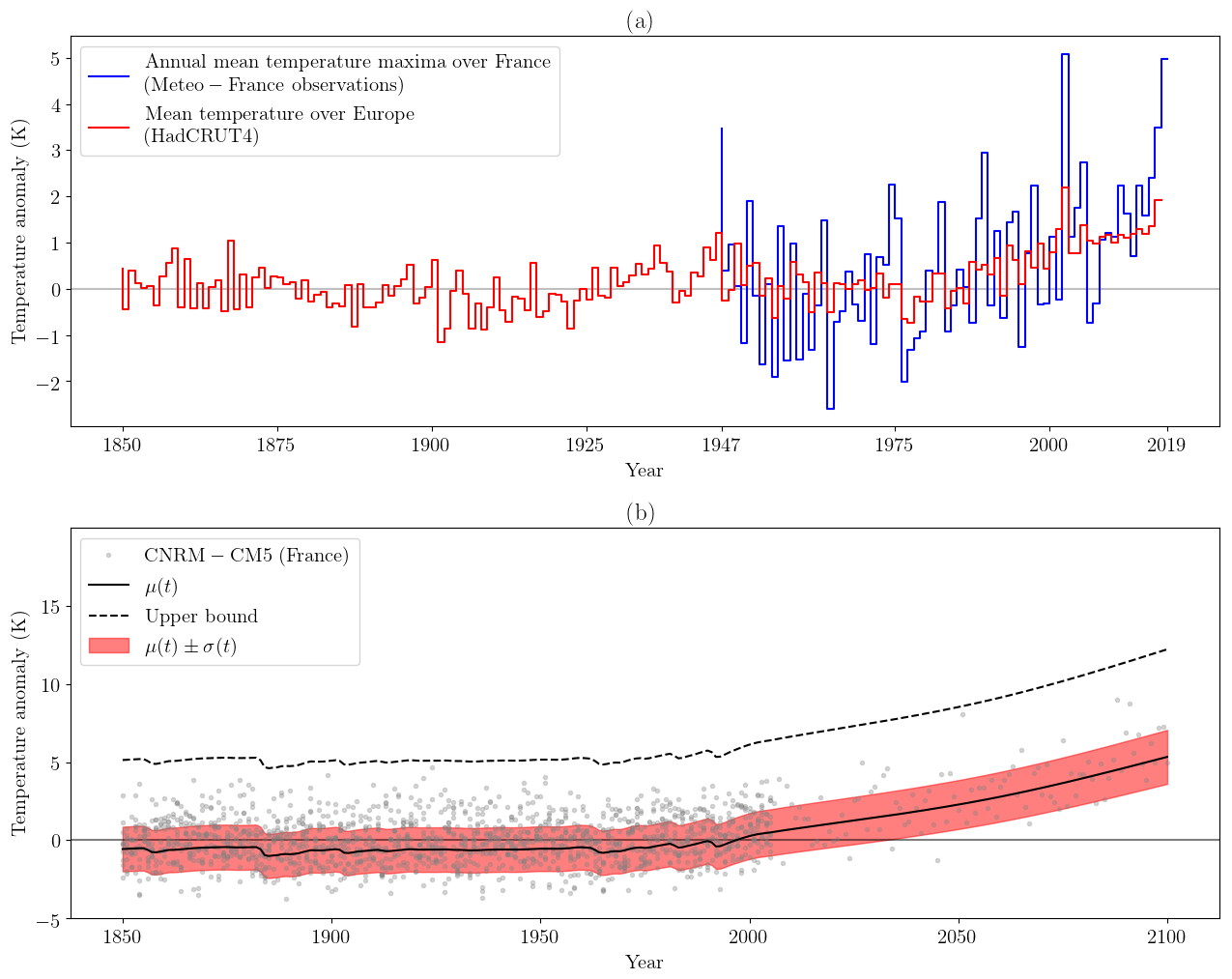
Figure 1(a) The red line shows the average of the mean temperature anomaly (with respect to 1961–1990) over Europe (35–70∘ N, 10∘ W–30∘ E), between 1850 and 2019, extracted from HadCRUT4 (Jones et al., 1999, 2001, 2012; Kennedy et al., 2011; Morice et al., 2012). The blue line shows the annual maxima of the anomaly (with respect to 1961–1990) with a 3 d moving average of thermal index over France, between 1947 and 2019 (30 stations over France, Météo-France data). (b) Example of a fit with a nonstationary GEV law (see Eq. 1) for the CNRM–CM5 model. The gray points are the values of the model over France. The black line is the location parameter μ(t). The red shading shows the scale parameters μ(t)±σ(t). The dotted black line is the upper bound, i.e., if ξ(t)<0.
2.1 Data set and event considered
To present our methodology, we propose implementing an attribution analysis of the extreme heat wave of July 2019. We focus on France (42–51∘ N, 5∘ W–10∘ E), and we consider the random variable of annual maxima of a 3 d average of the mean temperature anomaly with respect to the period 1961–1990, noted as T.
The time series of observations of T, denoted as To (note the difference between the random variable, which is a mathematical abstraction, and the realization, which is the observations), comes from the Météo-France thermal index. This index is built as an average of observations from 30 ground stations, showing data available between 1947 and 2019. The time series of To is represented in Fig. 1a. The annual 2019 maximum occurred in July during the heat wave. The anomaly of this event is equal to 4.98 K, slightly higher than the 2003 maximum (4.93 K; second highest).
Table 1List of CMIP5 models used in the literature (CMIP5, 2011; Taylor et al., 2012; Meehl et al., 2009; Hibbard et al., 2007).
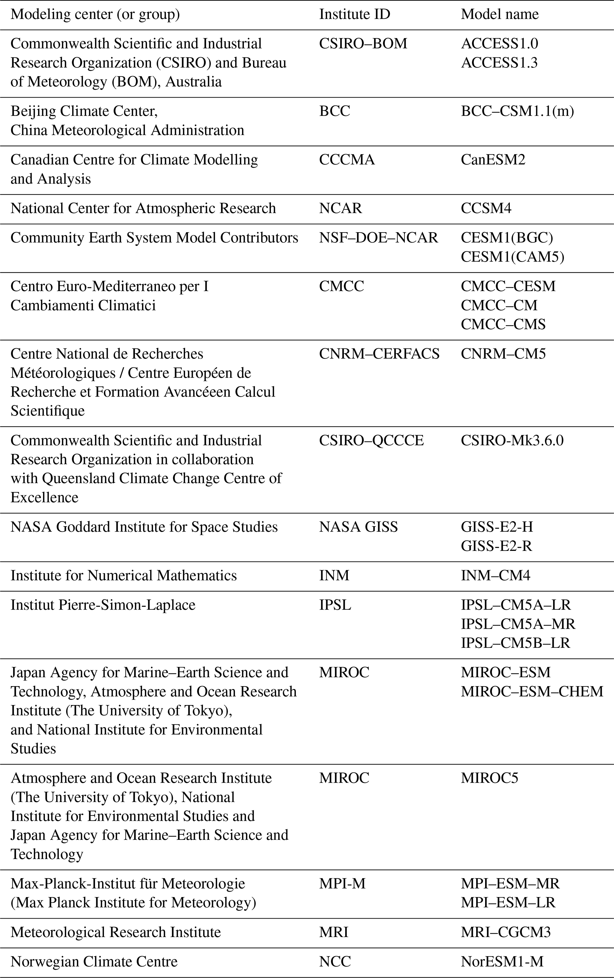
For climate models, we extract a simulated time series of T from the CMIP5 data set (CMIP5, 2011). We select all models for which simulations were produced between 1850 and 2100 and merge their historical runs with their representative concentration pathway 8.5 (RCP8.5; van Vuuren et al., 2011; Riahi et al., 2007) scenario simulations. All models selected are summarized in Table 1. In all, we have 26 climate models over France representing the random variable T.
We use the summer mean temperature anomaly with respect to period 1961–1990 over Europe as a covariate, noted as Xt, consistent with previous attribution studies (van Oldenborgh et al., 2015b; van der Wiel et al., 2017). For observations of the covariate, the data set HadCRUT4 (Jones et al., 1999, 2001, 2012; Kennedy et al., 2011; Morice et al., 2012) is used and noted as . For each CMIP5 model included in our analysis, we also extract this covariate by taking the mean temperature anomaly over Europe.
To summarize, we have the following:
-
The observation To of T, given by the Météo-France thermal index.
-
The observation of Xt, given by the HadCRUT4 data set.
-
A total of 26 time series of T from 26 CMIP5 models.
-
A total of 26 time series of Xt coming from 26 CMIP5 models.
2.2 Goal of attribution
A goal, in attribution, is to find the probability of the realization of the 2019 event, in the factual world (our world) and in the counterfactual world (without human influence). Noting and , the probability distribution of T in the factual and counterfactual world, respectively, we are looking for the following probabilities:
Observe the dependence in time of and . It is justified by the anthropic and natural forcings (such as volcanic eruptions) which alter the probability distribution with time. From the two probability distributions, we can also derive the intensity of the event. Noting and , the quantile functions, the intensity and in the factual/counterfactual world are defined by the following:
Finally, the attribution is performed with the two following indicators, namely the probability ratio and the change in intensity, which measure the influence of anthropic forcing as follows:
Consequently, an attribution study requires knowing the probability distribution and . The next sections describe the statistical model and how to use the climate models to infer these distribution with a Bayesian approach.
3.1 Statistical models
Classically, for the maximum temperature, the random variable T is assumed following a generalized extreme value distribution, in which parameters vary with a covariate Xt (either linearly or through a link function), depending on time and describing the response to external forcings. Mathematically we write that , as follows:
The parameters μ(t), σ(t) and ξ(t) are, respectively, the location (similar to the mean), scale (similar to the variance) and shape parameters. μ0, σ0 and ξ0 are called the stationary parameters, while μ1, σ1 and ξ1 are called the nonstationary parameters. The exponential link function is used for the scale parameter to ensure its positivity. We note this model . Note that several studies assume that (see e.g., van Oldenborgh et al., 2015b; van der Wiel et al., 2017), and we will test this hypothesis in the next section.
In the literature, the covariate Xt is assumed given by a 4-year moving average of the global mean surface temperature (GMST; see e.g., van Oldenborgh et al., 2015b; van der Wiel et al., 2017). Here, we take the forced component of the European summer mean temperature, which takes into account the regional and seasonal effect of aerosols. Then, we estimate the value of this covariate in the factual world, i.e., in response to all external forcings, denoted as , and in the counterfactual world, in response to natural forcings only, denoted as . Ribes et al. (2020) have shown a large uncertainty in the inference of Xt through the climate models and have proposed a method for considering uncertainty in the covariate Xt. Following their strategy in the GEV case, we define the random variable θ as follows:
The inference of the probability distribution of θ allows us to know the probability distributions and just by replacing the covariate Xt with and , respectively, in Eq. (1). Note that we assume that the coefficients and ξ1 are the same in the factual and counterfactual world; only the value of Xt differs between these two worlds.
Our goal is to infer the probability distribution of θ and to constrain it with Bayesian techniques by the observations and To. Mathematically, we want to derive the posterior of the following:
Our strategy is as follows. First, we estimate θ in each individual climate model considered. Second, we use the ensemble of climate models, in particular the spread in the estimated values, to derive a prior for the real-world value of θ. Third, we apply Bayesian techniques to derive the posterior of θ given observations of and observations To of T.
3.2 The covariate in the factual and counterfactual worlds
Here, we estimate the covariate Xt, i.e., the forced response of European summer mean temperature, for each single climate model over the period 1850–2100. This approach implies some uncertainty in the value of Xt. Indeed, the value of Xt is noise by the internal variability, and there is no link between the internal variability of Xt and that of T. This is done following the Ribes et al. (2020) approach closely, and it provides estimates of and . Our goal is to find the forced response from Xt, which requires a smoothing procedure. A generalized additive model (GAM; see e.g., Tibshirani, 1990) is used to decompose the time series of Xt as follows:
where
-
X0 is a constant,
-
is the response to natural forcings only (such as volcanoes) and is inferred from an energy balance model (Held et al., 2010; Geoffroy et al., 2013),
-
is the response to anthropogenic forcings; it is assumed to be a smooth function of time and is estimated using a smoothing procedure,
-
ε is a Gaussian random term due to internal variability.
Each of these terms has been estimated, and the response of Xt to external forcings in the factual and counterfactual worlds is easy to derive, as follows:
Furthermore, a covariance matrix is associated with the GAM decomposition in Eq. (3), describing the uncertainty of X0, and (i.e., the covariance matrix of X0, the linear regression coefficient involved in and the splines coefficients involved in ). We use it to draw 1000 perturbed realizations of the pair to describe their probability distribution.
We have represented, in Fig. S1, the two covariates and their respective uncertainty for three climate models. We can see different behaviors, with the model MIROC–ESM–CHEM increasing to +8 K at the end of the 21st century in the factual world, whereas the two others are between 4 and 5 K. Over the historical period, the CNRM model stays flat, whereas the two others increase or decrease. By anticipating a little, the synthesis of models shown in Fig. 4a and b depict a large range of uncertainty, justifying taking the uncertainty in the covariate into account.
This procedure (decomposition and perturbed realizations) is applied to each of the 26 realizations Xt from our CMIP5 models. Thus, at this step, we have inferred 26 distributions of the coupled , which is a subdistribution of our target θ. The next step involves fitting GEV models to each climate model and selecting the most appropriate statistical model.
3.3 Selection of the GEV model
We start by defining four submodels of Eq. (1), namely ℳμ,σ, ℳμ,ξ, ℳμ and ℳ0, which assume, respectively, that ξ1≡0, σ1≡0, and . We want to determine which GEV model out of , ℳμ,σ, ℳμ,ξ, ℳμ and ℳ0 is the most relevant. We propose using a likelihood ratio test (LRT) from theorem 2.7 of Coles et al. (2001). We start from two models, ℳa and ℳb, such that ℳa is a submodel of ℳb, and we note k as being the number of supplementary parameters in ℳb with respect to ℳa. For example, if ℳa=ℳμ, then k=1. The likelihood ratio test rejects ℳa in favor of ℳb at the significance level α if, in the following:
where l is the maximum of the log-likelihood function, and cα is the 1−α quantile of the k degree of freedom distribution. We propose identifying the best common GEV model by increasing the complexity by 1 degree of freedom at a time, i.e., k≡1. The pairs of models tested are represented as a tree in Fig. 2. Each edge of the tree is a test in which the left model represents ℳa, while the right model represents ℳb.
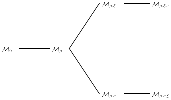
Figure 2Tree representing the likelihood ratio test (LRT) performed in Sect. 3.3. The variable ℳ0 is the GEV model with stationary parameters, and the variable ℳμ is the model where μ is nonstationary, etc. Each edge of the tree indicates a likelihood ratio test of the new model on the right of the edge, compared to the old model on the left of the edge.
The parameters of all GEV model are fitted from the realizations of T for each CMIP5 model, with the associated covariate from the GAM decomposition, using the maximum likelihood estimation (MLE). More details about the fit are given in Appendix A.
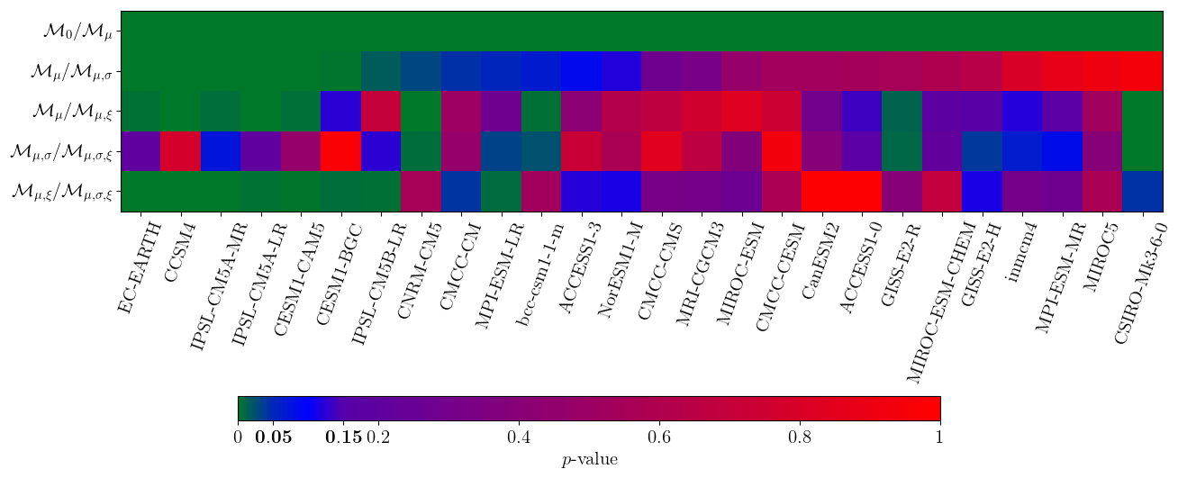
Figure 3Results of likelihood ratio test (LRT) to find which GEV model can be used for each CMIP5 model (x axis). ℳ0 is the stationary GEV model. ℳμ is the GEV model where μ is nonstationary, etc. The y axis labels indicate the test of the right model against the left model (see Fig. 2). For example, the first line test is if ℳμ (right) is more adapted than ℳ0 (left). The color map gives the p value of the LRT. A value higher than 0.15 (red) indicates that the new model is rejected. A value lower than 0.05 (green) indicates that the new model is accepted. The values between 0.05 and 0.15 (blue) are discussed in Sect. 3.3.
Results of our GEV model selection procedure are shown in Fig. 3 in the form of LRT p values. Low p values indicate that ℳa is rejected in favor of ℳb (green), i.e., a parameter has to be added. High p values suggest ℳa is suitable (red). p values between 0.05 and 0.15 (blue) are considered to give limited evidence.
First, all models agree with the consideration that μ must be nonstationary (the first line is very close to 0). This result is expected because the climate change signal in the RCP8.5 scenario is very high and directly alters the trend. Results are less obvious for other parameters. A total of seven CMIP5 models do not show evidence of any other form of nonstationarity, while 14 models suggest that either the scale or the shape are nonstationary. A total of eight (respectively, four) of these models suggest that the scale (respectively, shape) is nonstationary. For the two other models, it is not clear if the scale and shape must be simultaneously nonstationary or if we have a transfer of information between these two parameters.
Overall, these results suggest that we have to take into account a nonstationarity in the trend and in the scale or the shape. Because the MLE can swap information between the scale and the shape, and a small error of estimation in the shape can have a big impact on the fit, we choose to select the model ℳμ,σ. So, in the rest of this paper, we assume that ξ1≡0, and our nonstationary GEV model is written as follows:
Consequently, θ is now written as follows:
We can now infer the probability distribution of θ for each CMIP5 model. A bootstrapping procedure is used for each climate model in which the variable T is resampled 1000 times, corresponding to the 1000 estimates of derived from the previous section. Thus, 1000 perturbed , , , and are estimated per CMIP5 model. The goodness of fit of this model is assessed using a Kolmogorov–Smirnov test (see Fig. S2 and Table S1 in the Supplement) and shows a good agreement with the CMIP5 models. The best fit is shown in Fig. 1b for the CNRM–CM5 model (Fig. S3 in the Supplement shows the distribution of all fitted parameters and exhibits a large variability). First, in that case, the shape parameter is negative, equal to −0.23, implying the existence of an upper bound. Second, the upper bound follows the trend, and an extreme event occurring in the future might have been impossible in the past.
At this stage, we have 26 distributions of θ – one for each CMIP5 model – modeling the uncertainty of the covariates and the GEV parameters. Uncertainty of each distribution is quantified through a sample of 1000 bootstrapped parameters. We now focus on how to merge them into a single distribution representing multimodel uncertainty.
3.4 Deriving a prior from an ensemble of models
The goal is to synthesize our 26 distributions of θ into one single multimodel distribution. In a nutshell, we assume that each single model θ is a realization of this multimodel distribution, which is a multivariate Gaussian law in the dimension of (251 years for factual/counterfactual world and 5 parameters for the GEV). This distribution is therefore representative of the model spread – which is usually much larger than the uncertainty resulting from estimating θ in a single model. We subsequently use the “models are statistically indistinguishable from the truth” paradigm (Annan and Hargreaves, 2010) and assume that this multimodel distribution is a good prior for the real-world value. In practice, this synthesis is made following Ribes et al. (2017); details are given in Appendix B.
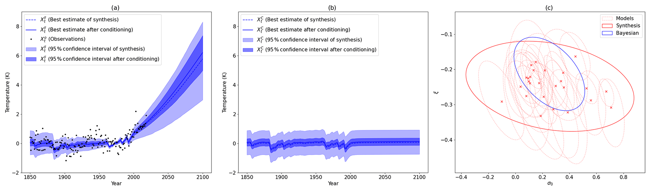
Figure 4(a) Covariate in the factual world. The dotted blue line and the blue line are the best estimate of the multimodel synthesis before and after applying the Bayesian constraint, respectively. The shading in light blue and dark blue are the 95 % confidence interval of the multimodel synthesis before and after Bayesian constraint, respectively. (b) Covariate in the counterfactual world. The dotted blue line and the solid blue line are the best estimate of the multimodel synthesis before and after applying the Bayesian constraint, respectively. The shading in light blue and dark blue are the 95 % confidence interval of the multimodel synthesis before and after Bayesian constraint, respectively. (c) Ellipsis are the 95 % confidence interval given by the covariance matrix for the 26 CMIP5 models (dotted red), the multimodel synthesis before (solid red) and after (blue) Bayesian constraint. The crosses are the best estimate of the individuals models.
The effect of the multimodel synthesis is shown in Fig. 4. Panels (a) and (b) depict the synthesis of the covariates and , respectively. The dotted blue line is the best estimate, and the light blue shading is the 95 % confidence interval. These two panels show a large uncertainty across models for the covariates; note that the uncertainty is almost null between 1961 and 1990 because the models are given in anomalies with respect to this period. Panel (c) shows the covariance matrix of the distribution of (σ0,ξ) as ellipsis of the 95 % confidence interval. The dotted red ellipsis are the individual models, depicting many different behaviors. The solid red ellipsis is the multimodel synthesis, which includes almost all the best estimates from individual models.
So, with this approach, we obtain a good candidate θ for our Bayesian prior, described in Eq. (2), inferred from the climate models.
3.5 Using observations to derive a posterior
To derive the posterior of , we start by applying the Bayesian theorem, as follows:
In other words, to constrain θ by To and , we can, first, constrain θ by , and, second, constrain the new random variable by To. Note the two steps; the prior of θ derived in the previous section is used to infer . This new random variable is then used as a prior to derive the posterior of the constraint by To.
The posterior of is already computed and used by Ribes et al. (2020), under the name of CX constraint. This distribution is easy to derive because both θ and are assumed to follow Gaussian distributions, and is a subvector of θ, so the Gaussian conditioning theorem (see e.g., Eaton, 1983) applies, and also follows an explicit Normal law. The effect of the constraint is represented in Fig. 4a and b. The blue line is the constrained best estimate, and the blue shading is the new confidence interval. We can see a significant decrease in the confidence interval. In the historical period, the covariate is closer to 0, except during volcanic episodes. For the projection period, the signal is increased by removing the lowest covariates.
The last step is to draw from the posterior of the Eq. (6). To draw a θ fully constrained from the posterior, we use a Markov chain Monte Carlo (MCMC) method, namely the Metropolis–Hastings algorithm (Hastings, 1970). We propose, for each sampling, performing 10 000 iterations of the MCMC algorithm (see Appendix C), and we assume that the last 5000 samples are drawn from the posterior . We uniformly draw one θ among these 5000 values, and we consider it as our new parameter. We use the median of these posterior drawings as a best estimate (e.g., for the final indicators ΔI and PR). As example of the effect of the constraint, we have added in Fig. 4c the covariance matrix of the pairs of parameters (σ0,ξ) in blue. We can see the significant decrease in the uncertainty and the shift of the parameters.
3.6 Summary
Finally, we obtain set of nonstationary parameters of a GEV distribution from a multimodel synthesis. It is fully constrained via Bayesian techniques. We have a synthetic description of the variable T as a GEV law, with best estimates of the parameters of that law and 1000 bootstrapped samples characterizing uncertainty on these parameters. Furthermore, using the decomposition of the covariate Xt, we can switch between the factual and counterfactual worlds.
Once the parameters of the GEV distributions have been inferred, we can compute the cumulative distribution function at any time t and derive the instantaneous probability of our event in the factual world, denoted as , and in the counterfactual world, denoted as . The usual attribution indicators, such as the probability (or risk) ratio , the fraction of attributable risk and also the change in intensity ΔIt, can be derived consistently from our description of T.
4.1 About the statistical model
In the literature (see e.g., van Oldenborgh et al., 2015b; van der Wiel et al., 2017), it is assumed (i) that (forcings do no affect the variability and shape), (ii) the covariate Xt is given by the observations of the 4-year moving average of the global mean surface temperature or the European mean temperature, (iii) the GEV distribution is directly fitted with the observations To, and (iv) the GEV distribution fitted describes only the factual world, while the counterfactual world is defined as a particular time in the past (e.g., the year 1900). In other words, .
First, the main argument assumes that is the large uncertainty during the fit, but we have seen that the climate models can exhibit at least a σ1 that is significantly different from 0. The uncertainty can be due to the small size of To (73 realizations currently). Second, the uncertainty of the covariate Xt is not taken into account, while we were able to see that it was not negligible, including over the period when the observations are known. Third, the definition of the counterfactual world depends on the date selected as being representative of preindustrial conditions, e.g., 1900 by Vautard et al. (2019). In particular, the counterfactual world can be affected by some anthropogenic forcings already present at that time. Our approach allows us to take this into account.
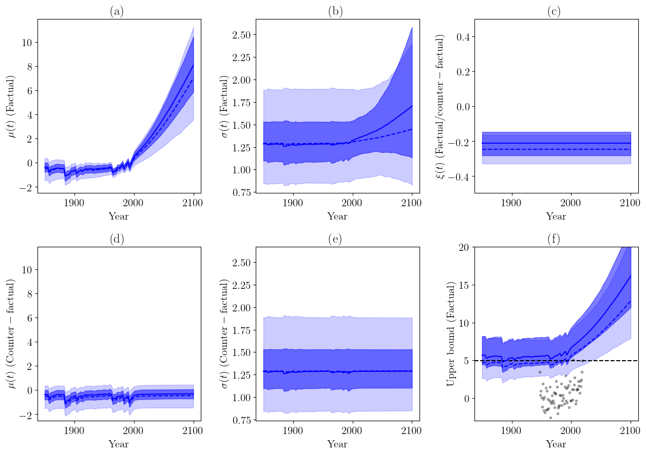
Figure 5GEV parameters μ(t), σ(t), ξ(t) and their uncertainty. Values in light blue describe the multimodel distribution, i.e., no observational constraint is applied. Values in dark blue illustrate the Bayesian constraint. The (dotted) blue lines are the best estimates, and the shading shows the 95 % confidence ranges. (a) Parameter μ(t) in a factual world. (b) Parameter σ(t) in a factual world. (c) Parameter ξ(t) in a (counter)factual world. (d) Parameter μ(t) in a counterfactual world. (e) Parameter σ(t) in a counterfactual world. (f) Upper bound of the fitted GEV distribution in the factual world, given by , if ξ(t)<0 or otherwise ∞. The black points are the observations, and the dotted black line is the maximal value of observations (in the year 2019).
4.2 About the constraint
In this section, we discuss the effect of the Bayesian constraint on GEV model parameters. The multimodel parameters and their confidence intervals are summarized in Fig. 5.
For the location parameter μ(t) in the factual world (Fig. 5a), we can see the trend of RCP8.5 simulations for each set of parameters. The effect of natural forcings is discernible over the period 1850–2000. The constraint tends to slightly reduce the confidence interval to between 40 % and 60 %. The best estimate of the change in μ(t) is slightly increased by the constraint, by about 0.5 K at the end of the 21st century. Note that in the counterfactual world (Fig. 5d) the trend is flat during the 21st century due to the absence of anthropogenic forcings in RCP scenarios over that period.
For the scale parameter in the factual world (Fig. 5b), application of the constraint leads to a large reduction in uncertainty by a factor of 2. A large trend in the scale becomes visible in the confidence interval over the 21st century. Note that the trend can be negative, or positive, corresponding to different climate models. No trend is visible in the counterfactual world (Fig. 5e). The Bayesian constraint suggests a much higher upward trend in σ(t).
Figure 5c shows the shape parameter, which is the same in the factual and the counterfactual worlds (the shape does not depend on the covariate). The shape, as estimated in the multimodel distribution, is always negative and is in the interval . Applying the Bayesian constraint, the uncertainty range is reduced to , with a best estimate equal to −0.2. An upper bound always exists in this case.
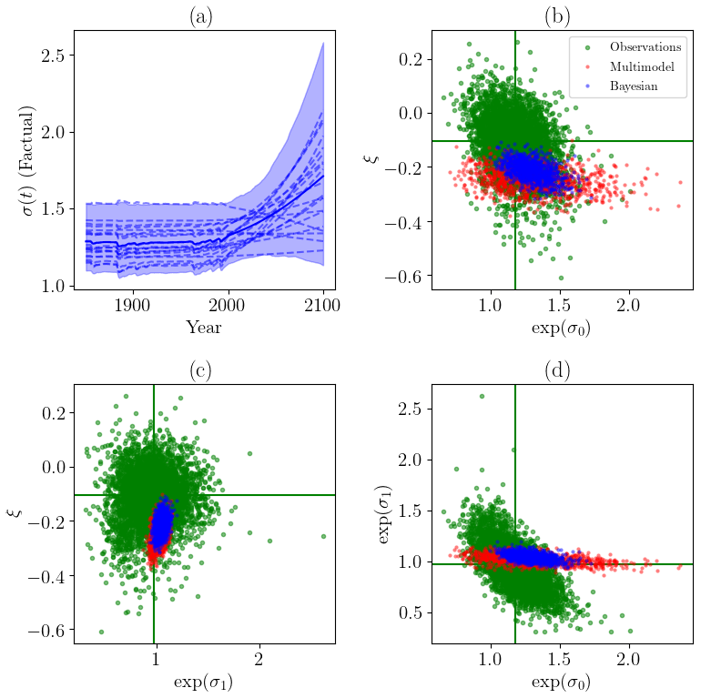
Figure 6(a) Examples of the sample of σ(t) after the Bayesian constraint. (b) Stationary scale parameters versus shape parameters for multimodel synthesis (red), Bayesian constraint (blue) and from observations (green). (c) Same as (b) but between nonstationary scale parameters and shape parameters. (d) Same as (b) but between stationary and nonstationary scale parameters.
We have represented, in Fig. 6, the parameters σ0,σ1 and ξ for the prior (i.e., the multimodel), the Bayesian constraints and for observations To. The parameters fitted for observations are derived from the same GEV model, and the covariate used is a spline smoothing of . The observed time series is bootstrapped 5000 times to sample the joint distribution between all three parameters. The Bayesian constraint is locked at the intersection between the prior and the observations. The prior and the distribution derived from observations often exhibit some overlap. This suggests that there is no clear evidence of observations being inconsistent with model-simulated parameters given the sampling uncertainty in observations, i.e., the difficulty in directly fitting a nonstationary GEV distribution to a very small sample (71 observations). We can also deduce that the prior has a relatively strong influence on the posterior; in particular, the range of σ0 is narrowed.
Figure 5f shows the upper bound of the fitted GEV distribution in the factual world. This bound is given by if the shape is negative and is infinite if the shape is positive. Here, the effects of the constraint are critical. In the unconstrained multimodel distribution, the estimated upper bound is sometimes lower than observed events; such events should be impossible, which suggests that this estimate is unreliable. After applying the constraint, the estimated upper bound is always higher than observations, consistent with expectations. Furthermore, we notice that the observed 2019 value is above plausible values of the GEV upper bound over the 19th and 20th centuries (i.e., within the confidence range), suggesting that the 2019 event might have had a null probability of occurring at that time.
Table 2Statistics of multimodel synthesis after Bayesian constraint in the years 2019 and 2040. The first column shows the statistics, the second the best estimate, the third the quantile 0.025 and the last the quantile 0.975.
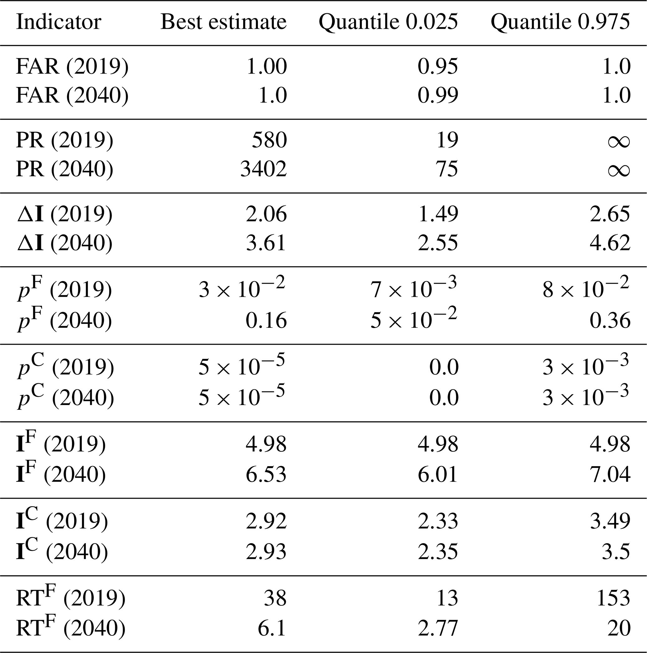

Figure 7(a) Probability ratio, , of multimodel synthesis after the Bayesian constraint. The gray line is the proportion of undetermined values (i.e., 0∕0). If the gray line is larger than 0.05 (the dotted gray line), the confidence interval is [0,∞]. The red shading is the 95 % confidence interval of undetermined values ( or ). The red line is the best estimate. (b) Change in intensity ΔIt, i.e., the difference between the value of an event with probability in a factual and counterfactual world for each year. The red shading is the 95 % confidence interval, and the red line is the best estimate.
4.3 About the heat wave
In this section, we discuss the attribution results derived from our methodology, based on the two indicators defined above. The first is the probability ratio , shown in Fig. 7a and b. The second is the change in intensity ΔIt between the factual and counterfactual worlds, shown in Fig. 7c and d. The statistics for the years 2019 and 2040 are summarized in Table 2, where is the factual world return time.
The probability ratio can be undetermined, e.g., if . In this case, if the proportion of undetermined values is greater than 0.05, we assume the confidence interval to be [0,∞] (∞ included). Specifically, the upper (respectively, lower) bound of the confidence interval is computed by assuming that all undetermined values are equal to ∞ (respectively, 0), corresponding to the least confident case. The proportion of undetermined values is indicated in gray along the timeline below each panel. After the 1990s, the ratio of undetermined values is lower than 0.05. We note that, to a certain extent, undetermined values indicate that the odds of the event have not changed (i.e., similar to PR=1) because the event is impossible in both the factual and the counterfactual worlds. The key point is that the heat wave is assessed as impossible in the factual and counterfactual worlds over the 19th and 20th centuries, with a probability between 5 % and 50 % particularly when volcanic eruptions occur.
Before 1990, the PR is not well defined, indicating no evidence of human influence on such an event. After 1990, the lower bound of the PR confidence interval increases quickly above 1. The probability of an event like the 2019 event is found to have increased by a factor in the range 19–∞ in 2019 and by a factor in the range 75–∞ in 2040. The value ∞ comes from realizations in which the event has a null probability in the counterfactual world. The estimated return time is in the range 13–153 years in 2019 and 3–20 years in 2040.
Estimated changes in intensity are consistent with the above picture. No change is detected before the year 1980, and then a sharp increase is found after that date, reaching ΔI to +2 K in the year 2019 (95 % confidence intervals of 1.5–2.7), which is consistent with the long-term climate change signal estimated over France in summer (currently nearing +2 K; see e.g., Ribes et al., 2016). According to the RCP8.5 scenario, the ΔI will continue to increase to 3.6 in 2040 (2.6–4.6). We note that the upper bound in the year 2100 is approaching +12 K, which corresponds to an annual maxima of mean temperature around 39 ∘C (29 ∘C in 2019).
4.4 About the world weather attribution (WWA) paper
We finish with a comparison to the fast attribution paper by Vautard et al. (2019, hereafter V19), who investigated the same event. V19 considers a T time series extracted from E-OBS observations (Cornes et al., 2018) and fits a GEV model with a nonstationary location parameter (a smoothed global mean temperature is used as a covariate) and a constant scale and shape. The method used to build confidence intervals has not been published, so the discussion below focuses on the best estimates.
V19 reports a return period of around 134 years (i.e., ), with a probability ratio at least equal to 10 and a change in intensity between 1.5 and 3 K from E-OBS. Results from CMIP5 models were rejected due to a scale parameter in models (=1.78, with uncertainty range [1.74, 1.83]) being in sharp disagreement with that estimated from E-OBS observations (1.08, with uncertainty range [0.81, 1.25]). Here, by making the best use of all available information, we find a return period between 13 and 153 years, a probability ratio at least equal to 19 and a change in intensity between 1.5 and 2.6.
Attribution results, i.e., PR and ΔI, agree reasonably well between the two studies. However, there is a substantial discrepancy in the estimated return time. We can propose some explanation for this discrepancy. (i) Our GEV model assumes a nonstationary scale parameter. In practice, we find a significant change in that parameter after the end of the 20th century, contributing to a shorter return time of the event. (ii) We use the entire historical record to apply our Bayesian constraint, while V19 excluded the observed 2019 value from their estimation procedure.
Another noticeable difference between these two studies involves the method of combining climate models and observations. For V19, the parameters of the GEV distribution are fitted from observations, and all models that are in disagreement (e.g., scale parameter too far) are rejected. They assume that the climate models rejected are lacking some physical process vital for the generation of extremes in the real world. We, instead, are assuming that the physical processes are there but potentially misrepresented in some way. After exploring the model uncertainty comprehensively, we find no inconsistency between models and observations. We therefore derive parameter ranges which are consistent with these two sources of information. In the end, model data do not play the same role in these two studies.
In this paper, we propose an extension of the method of Ribes et al. (2020), which was designed for Gaussian variables, for the analysis of extreme events and, in particular, generalized extreme value distributions. This extension can be used as soon as the event is sufficiently extreme under both the factual and counterfactual worlds in which the GEV modeling is applicable. We also provide new insights on observational constraints for attribution, and a new constraint based on Bayesian techniques is developed. This approach shows a good capacity to restrict the CMIP5 multimodel distribution to trajectories which are consistent with the observed time series. This method is applied to annual maxima of a 3 d moving average over France, with a focus on the July 2019 heat wave.
This method illustrates how CMIP5 models can be used to estimate the human influence on extremely hot events. A key point is the nonstationarity of the scale parameters, which is often assumed to be constant. Some CMIP5 models exhibit a strong change in this parameter. For a small subset of these models, the shape parameters could also be nonstationary. Over the observed period, such changes are limited and hidden by internal variability, so they cannot be ruled out by the observational constraint.
Potentially, our new method can be applied to any variable by just considering the maxima. Illustrating the potential of this technique on another type of extreme event, such as extreme rainfall, is an important area of exploration for future work. Examining the response of hot extremes to climate change in the new generation of climate models (CMIP6) would also be an attractive approach for assessing the nonstationarity of the scale and shape parameters from a broader ensemble.
The goal of this section is to explain how the coefficients of the model in Eq. (1) can be fitted. Classically, in a stationary context the parameters can be explicitly inferred with L moment estimators (Hosking et al., 1985; Hosking, 1990; Wang, 1996). Here, because we are in a nonstationary context, we have to use the maximum likelihood estimation (MLE). Given the density of the GEV distribution and , the time series to be fitted, we want to minimize over θ the negative log-likelihood function as follows:
This minimization cannot be solved explicitly, and we use the classic algorithm of Broyden–Fletcher–Goldfarb–Shanno (BFGS; Nocedal and Wright, 2006). This method is a gradient method (with an estimation of the Hessian matrix), and requires a starting point to converge to the solution. The gradient can be explicitly written as follows:
We focus on selecting the starting point. Classically, the L-moment estimators are used to initialize μ0, σ0 and ξ0, and it is assumed, for the starting point, that . This choice, mostly if μ1 and σ1 are far from 0, can make the likelihood and/or its gradient undetermined at the starting point, leading to a failed minimization.
We propose using the following modification of the initialization. We perform a quantile regression (Koenker and Bassett, 1978; Koenker and Hallock, 2001), with the covariate Xt of T for quantiles from 0.05 to 0.95 by steps of 0.01. The Frish–Newton algorithm (Koenker and Ng, 2005) is used to solve the quantile regression problem. We have 91 samples per unit time. For each time, we compute the L moments and, with a least square regression, we find an estimation of the nonstationary L moments. Applying the equation of Hosking et al. (1985), we find a first approximation of μ, σ and ξ0. Now, with a final least square regression, we can find an estimation of θ and then use this estimate to initialize the BFGS algorithm.
The main hypothesis of this multimodel synthesis is the paradigm that models are statistically indistinguishable from the truth. Following Ribes et al. (2017), we note that θ∗ is the multimodel synthesis and μθ is the truth. We decompose any models θi as and , where μθ+μi is the mean of the model θi, Σu is the climate modeling uncertainty – assumed equal for each model – and Σi is the internal variability of the model θi. The paradigm allows us to assume the following:
Taking , the multimodel mean, it follows:
Using our paradigm again, we have , so , and we find the following:
We have to find an estimator of Σu. The difference between an individual model and the multimodel mean is given by the following:
Consequently, it follows that:
An estimator of Σe is given by the moment method, by taking the empirical covariance matrix of all samples from all models. Thus, by noting +, the positive part of a matrix, we find finally, in the following:
In this section, we describe a Markov chain Monte Carlo method, namely the Metropolis–Hastings algorithm (Hastings, 1970). We have a random variable, X, with law ℙX parameterized by a set of parameters θ. It is assumed that θ is also a random variable, with law ℙθ, and we have an estimation of it. Finally, we also have an observation Xo of X. Our problem is constraining the law of θ, given the observation Xo. Mathematically, we want to draw samples from the posterior distribution ℙ(θ | Xo). Using Bayesian theorem, we can write the following:
Focus on the right term. The numerator is known; this is just the law ℙX and ℙθ, assumed known. The problem is the denominator because the law ℙ(Xo) is unknown. The Metropolis–Hastings algorithm starts with the following remark – for two realizations, θ0 and θ1, this ratio can be evaluated, and does it not depend on ℙ(Xo), as follows:
Thus, starting from a random θ0, a perturbation is applied to it, generating a θ1. The ratio ρ is computed, and if ρ>1, then θ1 is better than θ0 with respect to observations Xo, and it is accepted. Otherwise, a random number u is drawn from the uniform distribution in [0,1]. If ρ>u, then θ1 is accepted (and we accept a degradation) or else θ0 is kept. And this procedure is repeated. After a sufficiently large number of iterations, the sequence of θi generated is a Markov chain, drawing from the posterior distribution θ | Xo. Here, in Sect. 3.5, we wait 5000 iterations before drawing 5000 new samples from the posterior.
The CMIP5 database is freely available. Source codes realizing the GEV fit are freely available in the R Python package of SDFC under the CeCILL-C license (https://doi.org/10.5281/zenodo.4263886, Robin, 2020a). Source codes to reproduce the analysis of this article are packed into the library NSSEA under the CeCILL-C license (https://doi.org/10.5281/zenodo.4263904, Robin, 2020b).
The supplement related to this article is available online at: https://doi.org/10.5194/ascmo-6-205-2020-supplement.
YR performed the analyses. The experiments were codesigned by YR and AR. All the authors contributed to the writing of the paper.
The authors declare that they have no conflict of interest.
We acknowledge the World Climate Research Program (WCRP) Working Group on Coupled Modelling (WGCM), which is responsible for CMIP, and we thank the climate modeling groups (listed in Table 1 of this paper) for producing and making available their model output. For CMIP, the U.S. Department of Energy's Program for Climate Model Diagnosis and Intercomparison provided coordinating support and led the development of the software infrastructure in partnership with the Global Organization for Earth System Science Portals.
Part of this work was supported by the French Ministère de la Transition Énergétique et Solidaire, through the “Convention pour les Services Climatiques” grant, and the EUPHEME project, which is part of ERA4CS, an ERA-NET initiative by JPI Climate and cofunded by the European Union (grant no. 690462).
This paper was edited by Dan Cooley and reviewed by Daithi Stone and two anonymous referees.
Annan, J. D. and Hargreaves, J. C.: Reliability of the CMIP3 ensemble, Geophys. Res. Lett., 37, 2, https://doi.org/10.1029/2009GL041994, 2010. a
CMIP5: CLIVAR Exchanges – Special Issue: WCRP Coupled Model Intercomparison Project – Phase 5 – CMIP5, Project Report 56, available at: https://eprints.soton.ac.uk/194679/ (last access: 9 November 2020), 2011. a, b, c
Coles, S., Bawa, J., Trenner, L., and Dorazio, P.: An introduction to statistical modeling of extreme values, vol. 208, Springer Series in Statistics, Springer-Verlag, London, 2001. a
Cornes, R. C., van der Schrier, G., van den Besselaar, E. J. M., and Jones, P. D.: An Ensemble Version of the E-OBS Temperature and Precipitation Data Sets, J. Geophys. Res.-Atmos., 123, 9391–9409, https://doi.org/10.1029/2017JD028200, 2018. a
Eaton, M. L.: Multivariate statistics: a vector space approach, John Wiley & Sons, INC., 605 Third Ave., New York, NY 10158, USA, 1983, 512, 1983. a
Gabda, D., Tawn, J., and Brown, S.: A step towards efficient inference for trends in UK extreme temperatures through distributional linkage between observations and climate model data, Nat. Hazards, 98, 1135–1154, https://doi.org/10.1007/s11069-018-3504-8, 2019. a
Geoffroy, O., Saint-Martin, D., Bellon, G., Voldoire, A., Olivié, D. J. L., and Tytéca, S.: Transient Climate Response in a Two-Layer Energy-Balance Model. Part II: Representation of the Efficacy of Deep-Ocean Heat Uptake and Validation for CMIP5 AOGCMs, J. Climate, 26, 1859–1876, https://doi.org/10.1175/JCLI-D-12-00196.1, 2013. a
Hansen, G., Auffhammer, M., and Solow, A. R.: On the Attribution of a Single Event to Climate Change, J. Climate, 27, 8297–8301, https://doi.org/10.1175/JCLI-D-14-00399.1, 2014. a
Hastings, W. K.: Monte Carlo sampling methods using Markov chains and their applications, Biometrika, 57, 97–109, https://doi.org/10.1093/biomet/57.1.97, 1970. a, b
Held, I. M., Winton, M., Takahashi, K., Delworth, T., Zeng, F., and Vallis, G. K.: Probing the Fast and Slow Components of Global Warming by Returning Abruptly to Preindustrial Forcing, J. Climate, 23, 2418–2427, https://doi.org/10.1175/2009JCLI3466.1, 2010. a
Hibbard, K. A., Meehl, G. A., Cox, P. M., and Friedlingstein, P.: A strategy for climate change stabilization experiments, Eos, Transactions American Geophysical Union, 88, 217–221, https://doi.org/10.1029/2007EO200002, 2007. a
Hosking, J. R. M.: L-Moments: Analysis and Estimation of Distributions Using Linear Combinations of Order Statistics, J. Royal Stat. Soc.-Ser. B, 52, 105–124, 1990. a
Hosking, J. R. M., Wallis, J. R., and Wood, E. F.: Estimation of the Generalized Extreme-Value Distribution by the Method of Probability-Weighted Moments, Technometrics, 27, 251–261, https://doi.org/10.1080/00401706.1985.10488049, 1985. a, b
Jones, P. D., New, M., Parker, D. E., Martin, S., and Rigor, I. G.: Surface air temperature and its changes over the past 150 years, Rev. Geophys., 37, 173–199, https://doi.org/10.1029/1999RG900002, 1999. a, b
Jones, P. D., Osborn, T. J., Briffa, K. R., Folland, C. K., Horton, E. B., Alexander, L. V., Parker, D. E., and Rayner, N. A.: Adjusting for sampling density in grid box land and ocean surface temperature time series, J. Geophys. Res.-Atmos., 106, 3371–3380, https://doi.org/10.1029/2000JD900564, 2001. a, b
Jones, P. D., Lister, D. H., Osborn, T. J., Harpham, C., Salmon, M., and Morice, C. P.: Hemispheric and large-scale land-surface air temperature variations: An extensive revision and an update to 2010, J. Geophys. Res.-Atmos., 117, D5, https://doi.org/10.1029/2011JD017139, 2012. a, b
Kennedy, J. J., Rayner, N. A., Smith, R. O., Parker, D. E., and Saunby, M.: Reassessing biases and other uncertainties in sea surface temperature observations measured in situ since 1850: 2. Biases and homogenization, J. Geophys. Res.-Atmos., 116, D14, https://doi.org/10.1029/2010JD015220, 2011. a, b
Koenker, R. and Bassett, G.: Regression Quantiles, Econometrica, 46, 33–50, 1978. a
Koenker, R. and Hallock, K. F.: Quantile Regression, J. Econ. Persp., 15, 143–156, https://doi.org/10.1257/jep.15.4.143, 2001. a
Koenker, R. and Ng, P.: A Frisch-Newton Algorithm for Sparse Quantile Regression, Acta Math. Appl. Sin., 21, 225–236, https://doi.org/10.1007/s10255-005-0231-1, 2005. a
Meehl, G. A., Goddard, L., Murphy, J., Stouffer, R. J., Boer, G., Danabasoglu, G., Dixon, K., Giorgetta, M. A., Greene, A. M., Hawkins, E., Hegerl, G., Karoly, D., Keenlyside, N., Kimoto, M., Kirtman, B., Navarra, A., Pulwarty, R., Smith, D., Stammer, D., and Stockdale, T.: Decadal Prediction, B. Am. Meteorol. Soc., 90, 1467–1486, https://doi.org/10.1175/2009BAMS2778.1, 2009. a
Morice, C. P., Kennedy, J. J., Rayner, N. A., and Jones, P. D.: Quantifying uncertainties in global and regional temperature change using an ensemble of observational estimates: The HadCRUT4 data set, J. Geophys. Res.-Atmos., 117, D8, https://doi.org/10.1029/2011JD017187, 2012. a, b
Nocedal, J. and Wright, S.: Numerical optimization, 2, Springer Science & Business Media, Springer, New York, NY, https://doi.org/10.1007/978-0-387-40065-5, 2006. a
Otto, F. E. L., van der Wiel, K., van Oldenborgh, G. J., Philip, S., Kew, S. F., Uhe, P., and Cullen, H.: Climate change increases the probability of heavy rains in Northern England/Southern Scotland like those of storm Desmond – a real-time event attribution revisited, Environ. Res. Lett., 13, 024006, https://doi.org/10.1088/1748-9326/aa9663, 2018. a
Pall, P., Aina, T., Stone, D. A., Stott, P. A., Nozawa, T., Hilberts, A. G., Lohmann, D., and Allen, M. R.: Anthropogenic greenhouse gas contribution to flood risk in England and Wales in autumn 2000, Nature, 470, 382–385, 2011. a
Philip, S., Kew, S. F., Jan van Oldenborgh, G., Aalbers, E., Vautard, R., Otto, F., Haustein, K., Habets, F., and Singh, R.: Validation of a Rapid Attribution of the May/June 2016 Flood-Inducing Precipitation in France to Climate Change, J. Hydrometeorol, 19, 1881–1898, https://doi.org/10.1175/JHM-D-18-0074.1, 2018. a
Rahmstorf, S. and Coumou, D.: Increase of extreme events in a warming world, P. Natl. Acad. Sci. USA, 108, 17905–17909, https://doi.org/10.1073/pnas.1101766108, 2011. a
Riahi, K., Grübler, A., and Nakicenovic, N.: Scenarios of long-term socio-economic and environmental development under climate stabilization, Technol. Forecast. Soc. Change, 74, 887–935, https://doi.org/10.1016/j.techfore.2006.05.026, 2007. a
Ribes, A., Corre, L., Gibelin, A.-L., and Dubuisson, B.: Issues in estimating observed change at the local scale – a case study: the recent warming over France, Int. J. Climatol., 36, 3794–3806, https://doi.org/10.1002/joc.4593, 2016. a
Ribes, A., Zwiers, F. W., Azaïs, J.-M., and Naveau, P.: A new statistical approach to climate change detection and attribution, Clim. Dynam., 48, 367–386, https://doi.org/10.1007/s00382-016-3079-6, 2017. a, b
Ribes, A., Thao, S., and Cattiaux, J.: Describing the relationship between a weather event and climate change: a new statistical approach, J. Climate, 33, 6297–6314, https://doi.org/10.1175/JCLI-D-19-0217.1, 2020. a, b, c, d, e, f, g, h
Robin, Y.: yrobink/SDFC: SDFC_v0.5.0 (Version v0.5.0), Zenodo, https://doi.org/10.5281/zenodo.4263886, 2020. a
Robin, Y.: yrobink/NSSEA: NSSEA_v0.3.1 (Version v0.3.1), Zenodo, https://doi.org/10.5281/zenodo.4263904, 2020b. a
Stott, P. A., Stone, D. A., and Allen, M. R.: Human contribution to the European heatwave of 2003, Nature, 432, 610–614, https://doi.org/10.1038/nature03089, 2004. a
Taylor, K. E., Stouffer, R. J., and Meehl, G. A.: An Overview of CMIP5 and the Experiment Design, B. Am. Meteorol. Soc., 93, 485–498, https://doi.org/10.1175/BAMS-D-11-00094.1, 2012. a
Tibshirani, R. J.: Generalized additive models, Chapman and Hall, London, 1990. a
van der Wiel, K., Kapnick, S. B., van Oldenborgh, G. J., Whan, K., Philip, S., Vecchi, G. A., Singh, R. K., Arrighi, J., and Cullen, H.: Rapid attribution of the August 2016 flood-inducing extreme precipitation in south Louisiana to climate change, Hydrol. Earth Syst. Sci., 21, 897–921, https://doi.org/10.5194/hess-21-897-2017, 2017. a, b, c, d
van Oldenborgh, G. J., Haarsma, R., De Vries, H., and Allen, M. R.: Cold Extremes in North America vs. Mild Weather in Europe: The Winter of 2013–14 in the Context of a Warming World, B. Am. Meteorol. Soc., 96, 707–714, https://doi.org/10.1175/BAMS-D-14-00036.1, 2015a. a
van Oldenborgh, G. J., Otto, F. E. L., Haustein, K., and Cullen, H.: Climate change increases the probability of heavy rains like those of storm Desmond in the UK – an event attribution study in near-real time, Hydrol. Earth Syst. Sci. Discuss., 12, 13197–13216, https://doi.org/10.5194/hessd-12-13197-2015, 2015b. a, b, c, d
van Oldenborgh, G. J., Philip, S., Kew, S., van Weele, M., Uhe, P., Otto, F., Singh, R., Pai, I., Cullen, H., and AchutaRao, K.: Extreme heat in India and anthropogenic climate change, Nat. Hazards Earth Syst. Sci., 18, 365–381, https://doi.org/10.5194/nhess-18-365-2018, 2018. a
van Vuuren, D. P., Edmonds, J., Kainuma, M., Riahi, K., Thomson, A., Hibbard, K., Hurtt, G. C., Kram, T., Krey, V., Lamarque, J.-F., Masui, T., Meinshausen, M., Nakicenovic, N., Smith, S. J., and Rose, S. K.: The representative concentration pathways: an overview, Clim. Change, 109, 5, https://doi.org/10.1007/s10584-011-0148-z, 2011. a
Vautard, R., Boucher, O., van Oldenborgh, G. J., Otto, F., Haustein, K., Vogel, M. M., Seneviratne, S. I., Soubeyroux, J.-M., Schneider, M., Drouin, A., Ribes, A., Kreienkamp, F., Stott, P., and van Aalst, M.: Human contribution to the record-breaking July 2019 heatwave in Western Europe, available at: https://www.worldweatherattribution.org/human-contribution-to-the-record-breaking-july-2019-heat-wave-in-western-europe, last access: 19 September 2019. a, b, c
Vautard, R., van Aalst, M., Boucher, O., Drouin, A., Haustein, K., Kreienkamp, F., van Oldenborgh, G. J., Otto, F. E. L., Ribes, A., Robin, Y., Schneider, M., Soubeyroux, J.-M., Stott, P., Seneviratne, S. I., Vogel, M., and Wehner, M.: Human contribution to the record-breaking June and July 2019 heatwaves in Western Europe, Environ. Res. Lett., 15, 094077, https://doi.org/10.1088/1748-9326/aba3d4, 2020. a
Wang, Q. J.: Direct Sample Estimators of L Moments, Water Resour. Res., 32, 3617–3619, https://doi.org/10.1029/96WR02675, 1996. a
Wehner, M., Stone, D., Shiogama, H., Wolski, P., Ciavarella, A., Christidis, N., and Krishnan, H.: Early 21st century anthropogenic changes in extremely hot days as simulated by the C20C+ detection and attribution multi-model ensemble, Weather and Climate Extremes, 20, 1–8, https://doi.org/10.1016/j.wace.2018.03.001, 2018. a
Yiou, P. and Déandréis, C.: Stochastic ensemble climate forecast with an analogue model, Geosci. Model Dev., 12, 723–734, https://doi.org/10.5194/gmd-12-723-2019, 2019. a
- Abstract
- Introduction
- Event definition and general framework
- Description of the methodology
- Discussion
- Conclusions
- Appendix A: Fit the GEV model
- Appendix B: Multimodel synthesis
- Appendix C: Metropolis–Hastings algorithm
- Code and data availability
- Author contributions
- Competing interests
- Acknowledgements
- Financial support
- Review statement
- References
- Supplement