the Creative Commons Attribution 4.0 License.
the Creative Commons Attribution 4.0 License.
 | 17 Sep 2020
A new energy-balance approach to linear filtering for estimating effective radiative forcing from temperature time series
David B. Stephenson
Peter A. Stott
Reliable estimates of historical effective radiative forcing (ERF) are important for understanding the causes of past climate change and for constraining predictions of future warming.
This study proposes a new linear-filtering method for estimating historical radiative forcing from time series of global mean surface temperature (GMST), using energy-balance models (EBMs) fitted to GMST from CO2-quadrupling general circulation model (GCM) experiments. We show that the response of any k-box EBM can be represented as an ARMA(k, k−1) (autoregressive moving-average) filter. We show how, by inverting an EBM's ARMA filter representation, time series of surface temperature may be converted into radiative forcing. The method is illustrated using three-box EBM fits to two recent Earth system models from CMIP5 and CMIP6 (Coupled Model Intercomparison Project). A comparison with published results obtained using the established ERF_trans method, a purely GCM-based approach, shows that our new method gives an ERF time series that closely matches the GCM-based series (correlation of 0.83).
Time series of estimated historical ERF are obtained by applying the method to a dataset of historical temperature observations. The results show that there is clear evidence of a significant increase over the historical period with an estimated forcing in 2018 of 1.45±0.504 W m−2 when derived using the two Earth system models. This method could be used in the future to attribute past climate changes to anthropogenic and natural factors and to help constrain estimates of climate sensitivity.
- Article
(1353 KB) - Full-text XML
- BibTeX
- EndNote


The estimation of historical radiative forcing, a measure of the net change in the energy balance of the climate system in response to an external perturbation, is a matter of strong scientific interest, as evidenced by the dedication of a whole chapter to this topic in the most recent assessment report from the Intergovernmental Panel on Climate Change (IPCC) (Myhre et al., 2013). Historical radiative forcing; equilibrium climate sensitivity (ECS), the long-term increase in global mean surface temperature (GMST) caused by a doubling of atmospheric CO2 concentration; and transient climate response (TCR), the increase in GMST after 70 years of CO2 increasing at 1 % per year, are the three main quantities that inform long-range forecasts of global warming. Estimation of historical forcing is therefore of particular relevance to climate policy decision-makers. In this paper we develop a new method for estimating radiative forcing by inverting simple climate models, a method that can also be of benefit to the detection and attribution of climate change.
The term radiative forcing refers to a change in Earth's energy balance relative to some predefined baseline value, usually chosen to represent pre-industrial conditions. In this study we use the effective radiative forcing (ERF), whose definition is given in Myhre et al. (2013): “the change in net [top-of-the-atmosphere] downward radiative flux after allowing for atmospheric temperatures, water vapour and clouds to adjust, but with surface temperature or a portion of surface conditions unchanged.” The adjustments of atmospheric temperatures and other variables, included in the definition of ERF, are commonly referred to as “rapid adjustments” and take place over much shorter timescales than resultant changes in surface temperature (Vial et al., 2013; Chung and Soden, 2015; Smith et al., 2018).
It is infeasible to calculate historical radiative forcing from observational data using the raw definition of ERF, as relevant climate variables, in particular top-of-the-atmosphere (TOA) net downward radiative flux, were unobserved for most of the historical period. Techniques have therefore been developed for diagnosing radiative forcing from general circulation model (GCM) experiments. Forster et al. (2016) describe methods, such as ERF_trans, which use GCMs to simulate the historical period with and without emissions of various forcing agents and hence calculate associated changes in Earth's energy balance. Resulting series of estimated forcings are strictly conditional on the climate model used. This approach is computationally expensive, and there is also some unavoidable noise contamination of results due to internal variability in model output. More recently, Andrews and Forster (2020) have combined GCM simulations with instrumental observations of historical GMST and global heat uptake to constrain historical ERF.
Alternative approaches, based on simple climate models, have been used to estimate historical radiative forcing from the observational record (e.g. Tanaka et al., 2009; Urban and Keller, 2010; Padilla et al., 2011; Aldrin et al., 2012; Urban et al., 2014; Johansson et al., 2015; Ljungqvist, 2015). These studies used Bayesian inference (or non-linear Kalman filtering in the case of Padilla et al., 2011) to jointly estimate some or all of the parameters of a simple climate model together with corresponding series of historical forcing. A common aim of these studies is to constrain ECS, with uncertainty in ECS being found dependent on corresponding uncertainty in historical forcing (Tanaka et al., 2009). As well as being computationally cheaper, methods based on simple climate models have the appeal of directly incorporating observational data, as opposed to GCMs whose dependence on the historical record (through parameter tuning) can be more subtle.
The present study is motivated by the potential application of simple climate models and forcing estimation techniques to the detection and attribution problem. Simple climate models have previously been used for detection and attribution of changes in GMST (e.g. Otto et al., 2015; Rypdal, 2015; Haustein et al., 2017). These studies regressed time series of historical temperature observations on predicted temperature series from linear impulse-response models, thus applying a simplified version of the widely used optimal fingerprinting methodology (Hasselmann, 1997; Allen and Tett, 1999; Allen and Stott, 2003), which is more typically applied to high-dimensional gridded datasets of observations and GCM output.
In the context of detection and attribution, surface temperature is an observable proxy for radiative forcing, which is itself not directly observable. The suitability of this proxy for regression analysis is reduced by two artefacts of the climate system's thermal inertia: (i) a delayed temperature response to changes in radiative forcing and (ii) strong temporal autocorrelation in natural temperature variability. Within the framework of linear impulse-response models, instantaneous surface temperature is simply a convolution of previous changes in radiative forcing (Good et al., 2011). We therefore propose that detection and attribution of changes in GMST using simple climate models could be improved by first deconvolving temperature observations to obtain series of estimated radiative forcing and then by performing the traditional regression step on radiative-forcing time series. In this way we might reasonably expect to eliminate (or at least reduce) both the time delay in the regressed series and also the temporal autocorrelation in the regression residuals.
This paper is a proof-of-concept study in which we develop a method for performing the proposed deconvolution of temperature time series using k-box energy-balance models (EBMs). To do this, we exploit a known correspondence between linear ordinary differential equations (ODEs) and discrete-time autoregressive moving-average (ARMA) time series models. Specifically, we use the fact that a system of k first-order linear ODEs has a discrete-time representation as an ARMA(k, k−1) filter (Spolia and Chander, 1974; Chang et al., 1982). This correspondence has been used before in the context of three-box EBMs by Grieser and Schönwiese (2001) as a convenient means of integrating the continuous-time model over a time series of discrete forcing inputs and by Stern (2005) as a way to enforce energy-balance constraints on estimated parameters of an ARMA model.
Here we propose a novel application of the three-box EBM filter in its inverted form. Li and Jarvis (2009) showed that the three-box model is simply a physically motivated parameterization of a causal, linear input–output system which maps a time series of radiative forcings onto a corresponding time series of surface temperatures. In this paper we show how the k-box model's equivalent ARMA filter representation may be derived, and we describe how, by inverting the ARMA filter, radiative forcing may be obtained from a temperature time series.
An energy-balance model (EBM) is a simple climate model where the time evolution of global temperatures is explained by changes in Earth's radiative imbalance. The simplest class of EBM, known as the k-box (or k-layer) model, consists of two components.
Firstly, a linear relation between GMST anomaly T1 and TOA net downward radiative flux change N determines the equilibrium response to radiative forcing ℱ (Gregory et al., 2004). In its most basic form,
where κ1 denotes the “climate feedback” parameter, which is conventionally denoted by λ. The notation used here is consistent with Fredriksen and Rypdal (2017) and Cummins et al. (2020).
Secondly, a system of k vertically stacked boxes recreates the thermal inertia of the ocean mixed layer and deep ocean, determining the characteristic timescales over which the response unfolds (e.g. Gregory, 2000; Held et al., 2010; Geoffroy et al., 2013). For k=3:
where Ti and Ci denote the temperature and heat capacity of each box and κi controls the rate of heat transfer between boxes.
To account for temporal variation in the relationship between T1 and N, which is present in some climate model experiments, Eqs. (1) and (3) may be modified to include a so-called efficacy factor ε (Held et al., 2010). Equation (1) then becomes
while Eq. (3) becomes
Internal variability in surface temperature, i.e. fluctuations in T1 not attributable to changes in ℱ, may be modelled by adding a white-noise process to the right-hand side of Eq. (2) (Hasselmann, 1976). For a schematic diagram of the EBM described in this section, see Fig. 1.
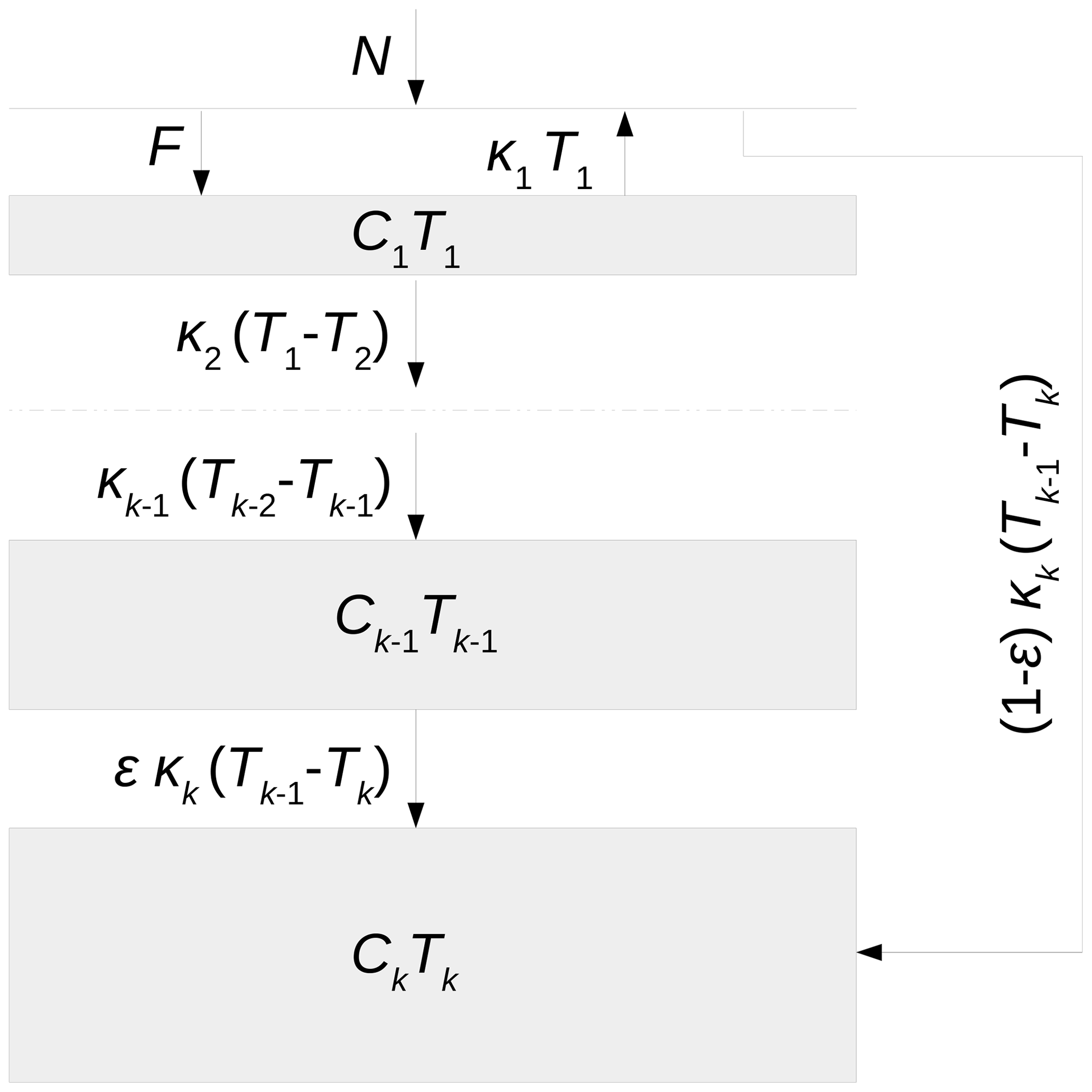
Figure 1Vertical layout of the boxes in the k-box energy-balance model. The thickness of each box indicates its heat capacity, and the arrows represent the flow of heat between adjacent boxes. The top of the atmosphere has no heat capacity and so is represented by a horizontal line. The dashed line in the middle is an abbreviation of the intervening boxes. See Cummins et al. (2020) for more discussion.
For a time-invariant linear system (such as the k-box model), the surface temperature response to a general forcing ℱ(t) can be written as
where R(v) is the discrete-time impulse-response function. Since an impulse is the derivative of a step change, the discrete-time impulse-response function is equal to the once-differenced response to a step change in forcing (e.g. a CO2-quadrupling experiment). Defining the “backshift” operator B such that , we can write
Let
It can be shown (see Appendix A) that for the k-box model
with ϕ and θ being polynomials in B of degree k and k−1 respectively. Thus we have
i.e. the linear map from ℱ(t) onto T1(t) is an ARMA(k, k−1) filter. The representation in Eq. (10) as a ratio of two polynomials gives us the corresponding inverse filter
which is ARMA(k−1, k). The AR (autoregressive) and MA (moving-average) coefficients can be efficiently calculated from the discrete-time impulse response using software for computing Padé approximants such as the “Pade” package in R (Adler, 2015).
Note that the above result for k-box EBMs is a special case of a long-standing and more general result: a system of k first-order linear ODEs has a discrete-time representation as an ARMA(k, k−1) filter (Spolia and Chander, 1974). EBM-derived ARMA filters have previously been used in the climate literature in the “forward” direction, i.e. to convert time series of annually averaged forcings into temperatures (Grieser and Schönwiese, 2001) and for the purpose of EBM parameter estimation (Stern, 2005). Here we apply the ARMA filter in the reverse direction, to find the forcing input required by an EBM to yield a given time series of temperatures.
Cummins et al. (2020) developed a maximum-likelihood method for estimating parameters of k-box EBMs from abrupt CO2-quadrupling GCM experiments. Using their method, three-box models have been fitted to the two most recent Earth system models (ESMs) from the UK Met Office: HadGEM2-ES (Hadley Centre Global Environmental Model) from CMIP5 (Coupled Model Intercomparison Project) and HadGEM3-GC3.1-LL from CMIP6 (see Fig. 2).
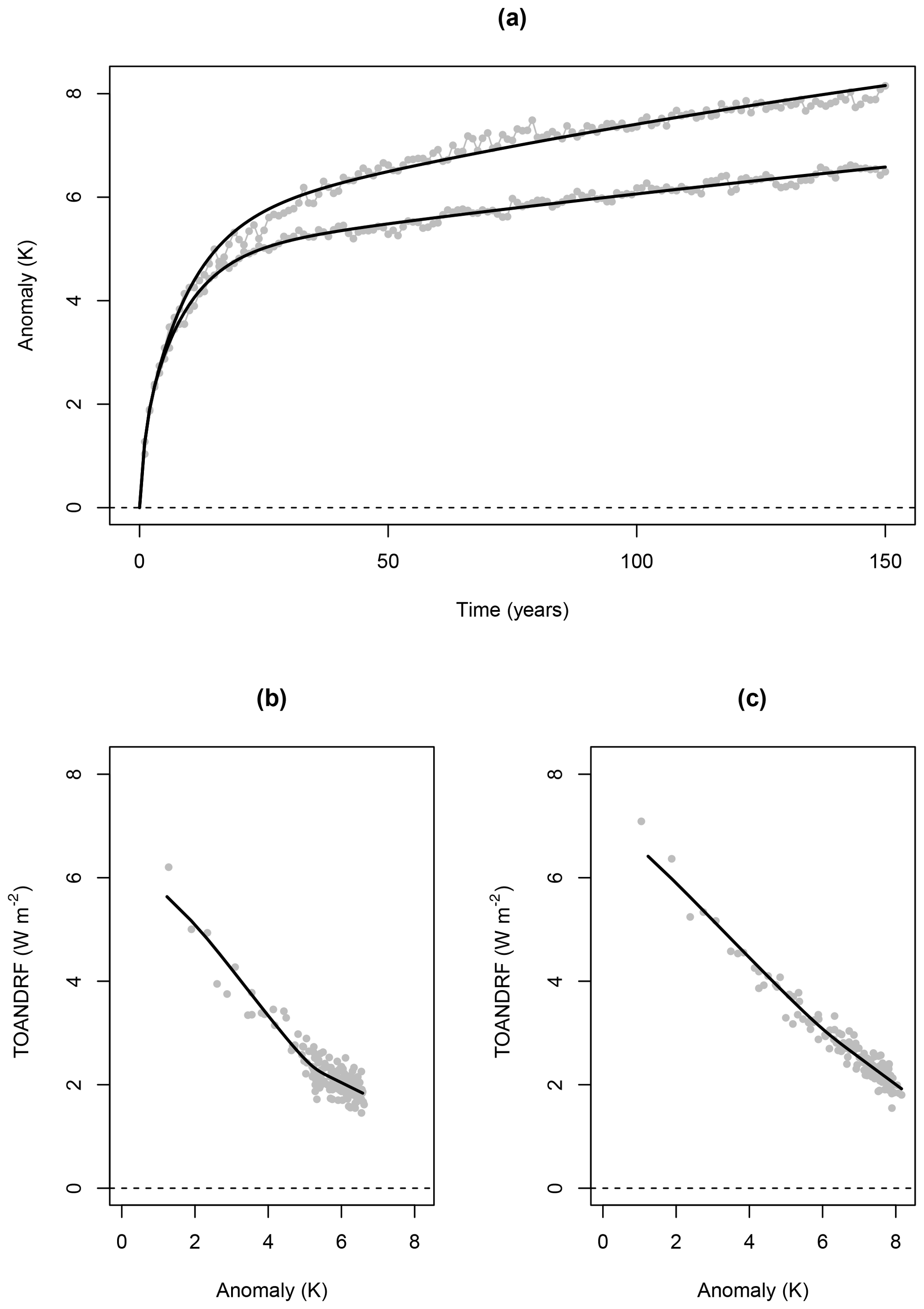
Figure 2Three-box model fitted values. Panel (a) shows the abrupt 4×CO2 surface temperature responses of the HadGEM2-ES (cooler) and HadGEM3-GC3.1-LL (hotter) climate models. Anomalies are relative to the time average of surface temperature in the corresponding pre-industrial control (piControl) simulations. Panels (b) and (c) show the TOA net downward radiative flux (TOANDRF) change in the respective models as a function of surface temperature.
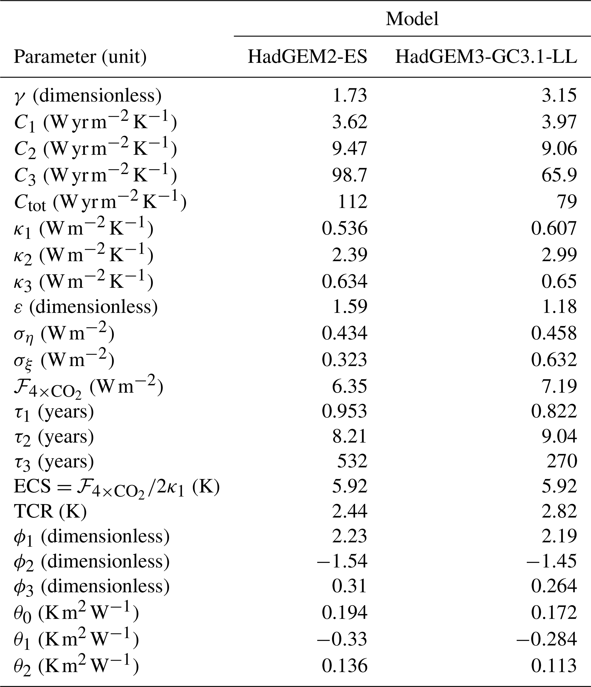
Table 1 contains maximum-likelihood estimates of model parameters, as well as estimates of equilibrium climate sensitivity (ECS); transient climate response (TCR); characteristic timescales τ1, τ2, and τ3; and the coefficients of the ARMA polynomials ϕ(B) and θ(B). The ARMA coefficients were calculated from the discrete-time impulse responses of the fitted models.
Table 1Maximum-likelihood parameter estimates. For descriptions of all model parameters, see Table 1 of Cummins et al. (2020). Note that parameters γ and ση are not used in this study. The values of ECS and TCR in this table are derived directly from the box models' physical parameters.
Note that ARMA models can alternatively be estimated using Bayesian inference (e.g. Monahan, 1983).
Numerical estimates of the ARMA coefficients enable, in theory, conversion of time series of surface temperatures into corresponding series of radiative forcings. The properties of this proposed temperature-forcing conversion were investigated using CMIP6 historical runs from the HadGEM3-GC3.1-LL climate model.
Model surface temperatures from 1850 to 2014 were averaged annually (January–December), globally and over four ensemble members. Anomalies were calculated by subtracting from the whole series the mean absolute temperature in the first 50 years (1850–1899). The final temperature series was fed into the fitted HadGEM3-GC3.1-LL ARMA filter using the digital filter implementation in the “signal” package in R (signal developers, 2014).
The resulting filtered forcing series was compared (see Fig. 3) with a time series of effective radiative forcing (ERF) diagnosed by Andrews et al. (2019) from a HadGEM3-GC3.1-LL RFMIP (Radiative Forcing Model Intercomparison Project) run1 using the ERF_trans method described in Forster et al. (2016). Note that Andrews et al. (2019) applied a time-mean historical volcanic forcing to the HadGEM3-GC3.1-LL piControl (pre-industrial control), meaning that they report an ERF of around 0.2 W m−2 in 1850. To avoid an offset due to our choice of temperature baseline, we add 0.2 W m−2 to the forcing series computed from the ARMA filter.
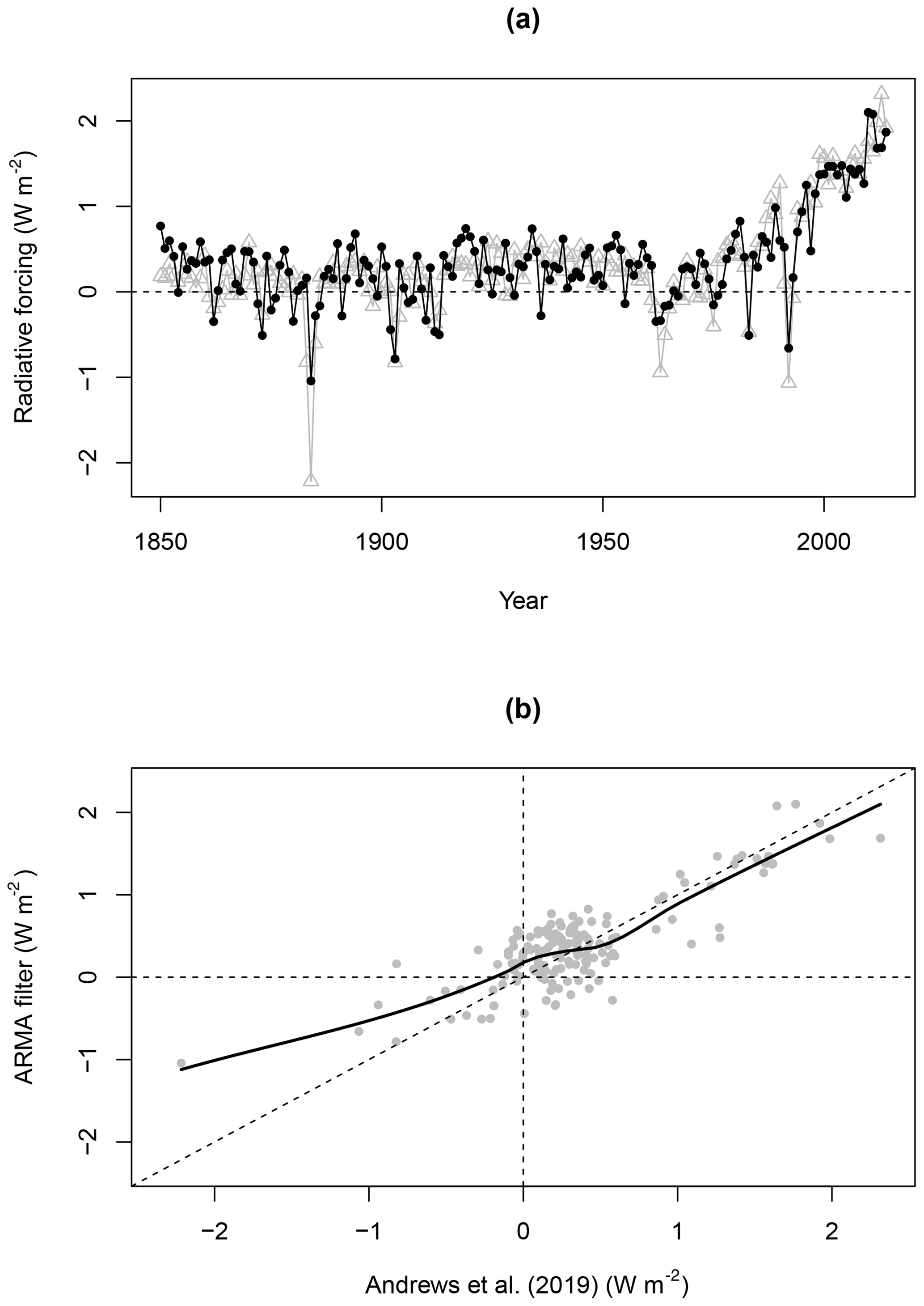
Figure 3Comparison of forcing series estimated from HadGEM3-GC3.1-LL simulations of the historical period. In panel (a) grey triangles denote forcings estimated by Andrews et al. (2019), while black dots denote forcings obtained using the three-box ARMA filter. Panel (b) shows how estimates from the two methods vary over the range of forcing values using a non-parametric curve fit. The diagonal line has equation y=x.
Results from the two methods agree strongly, and the filtered forcing series explains a majority of the variance in the ERF_trans series: the coefficient of determination is R2=0.69 (correlation of 0.83). Reassuringly the ARMA filter correctly infers the rate of forcing increase in recent decades. However, there appears to be a systematic disagreement in years with strong negative forcing. Negative forcing spikes associated with volcanic eruptions are smaller when calculated using the ARMA filter. This is especially evident in the case of Krakatoa (1883).
The observed discrepancy in inferred volcanic forcing is not entirely unexpected. The ARMA filter is derived from a three-box EBM which is known to be unable to resolve temperature responses on timescales significantly shorter than 1 year. Because the data used here are annual averages, there is also scope for error due to discretization, as a volcanic eruption might occur earlier or later in a given year. Finally, it may also be the case that the GCM's temperature response to volcanic forcing deviates from the linearity assumption of the ARMA filter.
By applying the box-model ARMA filters to time series of historical surface temperatures, we can obtain series of estimated historical forcings. The Cowtan and Way 2.0 (CW2.0) historical temperature series is an updated version of the dataset described in Cowtan and Way (2014), which is a modification of the HadCRUT4 (Hadley Centre Climatic Research Unit Temperature) series (Morice et al., 2012), corrected for coverage bias. Because CW2.0 is a blend of surface air temperatures (SATs) and sea surface temperatures (SSTs), it is not directly comparable with the pure-SAT 4×CO2 datasets used to calibrate the EBMs. The CW2.0 temperatures series have therefore been scaled by 1.09 according to Richardson et al. (2016) for use in this study. The HadGEM2-ES and HadGEM3-GC3.1-LL ARMA filters have been applied to the scaled CW2.0 temperatures2, yielding estimated historical forcing series for the period 1850–2018 (see Fig. 4).
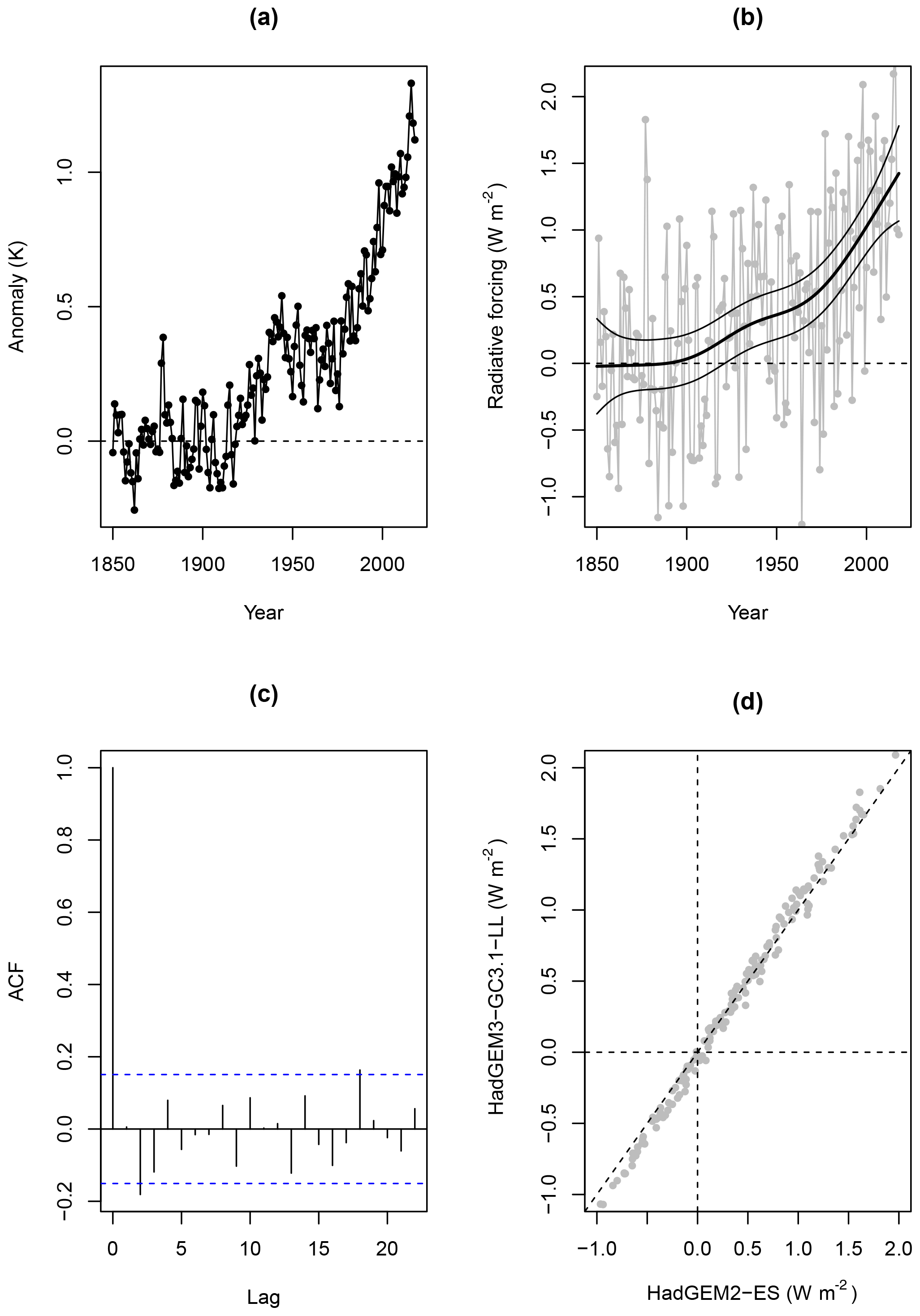
Figure 4HadGEM3-GC3.1-LL three-box ARMA filter reconstruction of historical radiative forcing. Panel (a) is the Cowtan and Way 2.0 temperature series; (b) is the corresponding filtered forcing series, with an estimated trend and 95 % confidence intervals from a generalized additive model (GAM) fit; (c) is the sample autocorrelation function (ACF) of the GAM residuals; (d) shows how estimates from the two models vary over the range of forcing values.
It can be seen from panel (d) of Fig. 4 that the forcing series generated by the two ARMA filters are very similar. The HadGEM3-GC3.1-LL ARMA filter reports slightly higher forcing in the latter years of the historical period and slightly more extreme negative forcing in years surrounding major volcanic eruptions.
The reconstructed forcing series are very noisy, since the natural variability which contaminates historical surface temperatures is amplified by the ARMA filter. However, unlike noise in the temperature series, the filtered noise is essentially uncorrelated in time. This follows from the fact that the three-box EBM successfully accounts for the thermal inertia (memory) of the system. The white-noise-like properties of natural variability in the filtered forcing series mean that the long-term trend can be extracted using regression techniques. A generalized additive model (GAM) was fitted to the estimated forcing series using the “mgcv” package in R (Wood, 2011). Approximate 95 % confidence intervals (±1.96 standard errors) for the estimated trend indicate a dramatic acceleration in radiative forcing in the second half of the twentieth century, with an estimated forcing increase of 1.45±0.504 W m−2 between 1850 and 2018.
The filtered forcing series and its subsequent decomposition into signal and noise are subject to multiple sources of uncertainty which must be taken into consideration. As well as the (substantial) internal climate variability, there is observational uncertainty in the historical temperature series and parameter uncertainty in the fitted impulse responses. Given a standard assumption of zero-mean errors, the aggregate noise from observational error and internal climate variability should be well accounted for by GAM regression smoothing. Uncertainty in the fitted impulse responses is also of limited concern: since the EBMs were fitted to abrupt CO2-quadrupling experiments, which have a good signal-to-noise ratio, uncertainty in the fitted impulse responses is in fact quite small (see Fig. 2). It should however be noted that, under forcing scenarios less drastic than 4×CO2, fitting of exponential response functions can suffer from ill-conditioning (De Groen and De Moor, 1987; Kaufmann, 2003). Of arguably greater concern is uncertainty due to inter-model variation between GCMs, which can be seen as a measure of confidence in a particular GCM's ability to represent the true climate. Inter-model variation in GCM output can arise through the use of different parameter values and/or model structures in GCMs (Flato et al., 2013). A full multi-model ensemble, perhaps across all the GCMs in CMIP6, would be required to quantify this satisfactorily, as HadGEM2-ES and HadGEM3-GC3.1-LL are clearly not independent samples. Our numerical results should therefore be seen as conditional on those two climate models.
While we argue that the use of a post hoc GAM regression is reasonable for the reasons given above, a more integrated approach to uncertainty quantification in future analyses might be achieved using Bayesian methods. A Bayesian alternative to GAM smoothing of the filtered forcing series is the “latent-force model” approach (Álvarez et al., 2009; Särkkä et al., 2018). In a latent-force model, uncertainty in the unobserved historical forcing input to a system of ODEs is represented in continuous time using a Gaussian process. Another alternative is the use of sequential methods based on the Kalman filter (Kalman, 1960). ARMA models have natural representations as linear Kalman filters (De Jong and Penzer, 2004), and sequential filtering methods can account for uncertainty in both model parameters and unknown inputs simultaneously, by augmenting the system state vector with estimates of the uncertain parameters (Lourens et al., 2012; Yu and Chakravorty, 2015). Similar techniques have previously been used in the climate literature: for example, by Annan et al. (2005) and Padilla et al. (2011), who used Kalman filtering to sequentially tune parameters of an Earth model of intermediate complexity (EMIC) and a two-box EBM respectively, and by Cohen and Wang (2014), who estimated historical time series of global black carbon emissions.
A framework has been developed for estimating radiative forcing from time series of surface temperatures using GCM-calibrated k-box EBMs. There is a known correspondence between k-box EBMs and ARMA models. We have shown how, by inverting a k-box EBM's equivalent ARMA filter representation, a convenient mapping from temperatures onto forcings may be obtained. The method has been validated using historical simulations from the HadGEM3-GC3.1-LL climate model and found to generally perform well, with the notable exception being negative forcing due to volcanic eruptions, which was underestimated. Three-box EBMs fitted to the HadGEM2-ES and HadGEM3-GC3.1-LL climate models have been combined with the Cowtan and Way 2.0 temperature dataset to produce estimates of radiative forcing for the historical period (1850–2018). Forcing estimates calculated using the two models' ARMA filters are very similar. A significant increase in radiative forcing over the historical period has been detected at the 95 % level.
This study has developed a method which has the potential to improve the detection and attribution of past temperature changes by comparing patterns of forcings rather than temperatures. Future work will examine how performance of the method generalizes to the other GCMs in CMIP6 and will address in more detail the question of uncertainty quantification. By combining ARMA filter estimates of historical radiative forcing with known observational constraints, it may be possible to further constrain climate sensitivity metrics, such as ECS and TCR, and hence constrain projections of future warming.
The step response of the k-box EBM is a linear combination of saturating exponentials (Geoffroy et al., 2013; Tsutsui, 2020; Cummins et al., 2020). The discrete-time impulse response R(v) is a linear function of the step response and is a sum of decaying exponentials:
where and . Then
It follows that the operator Φ(B) is a ratio of polynomials θ(B) and ϕ(B) of degree k−1 and k respectively. Cases k=1, 2, and 3 are shown below.
Case k=1
so ϕ(B) and θ(B) have respective degrees one and zero; i.e. the system is an ARMA(1, 0) or simply AR(1) filter.
Case k=2
so ϕ(B) and θ(B) have respective degrees two and one; i.e. the system is an ARMA(2, 1) filter.
Case k=3
so ϕ(B) and θ(B) have respective degrees three and two; i.e. the system is an ARMA(3, 2) filter.
Note that, in the statistics literature, the term “ARMA process” generally refers to an ARMA filter driven by a Gaussian white-noise input. For more information about ARMA models and the backshift operator, see Brockwell and Davis (2002).
The HadGEM2-ES and HadGEM3-GC3.1-LL surface temperature and TOA radiative flux datasets are available for download from Earth System Grid Federation (ESGF) portals, e.g. https://esgf-data.dkrz.de/ (last access: 6 December 2019). The time series of historical ERF for HadGEM3-GC3.1-LL estimated by Andrews et al. (2019) is available at https://doi.org/10.1029/2019MS001866 (https://github.com/timothyandrews/HadGEM3-ERF-Timeseries, last access: 10 December 2019). The Cowtan and Way 2.0 historical surface temperature series is available at https://www-users.york.ac.uk/~kdc3/papers/coverage2013/had4_krig_annual_v2_0_0.txt (last access: 29 November 2019) (Cowtan and Way, 2014).
All authors contributed to the development of the statistical methodology and the interpretation of the results. DPC performed the data analysis and was responsible for writing the paper. DBS and PAS proofread and edited the paper.
The authors declare that they have no conflict of interest.
We are grateful to Chris E. Forest and the anonymous referees for their useful comments. We thank Timothy Andrews of the Met Office Hadley Centre for providing forcing data for the HadGEM3-GC3.1-LL model, originally calculated in Andrews et al. (2019). We acknowledge the World Climate Research Programme's Working Group on Coupled Modelling, which is responsible for CMIP, and we thank the climate modelling groups for producing and making available their model output. For CMIP the US Department of Energy's Program for Climate Model Diagnosis and Intercomparison provides coordinating support and led development of software infrastructure in partnership with the Global Organization for Earth System Science Portals. David B. Stephenson wishes to thank Richard E. Chandler for a helpful discussion about the AR representation of an exponential MA response at the 14th International Meeting on Statistical Climatology.
This paper was edited by Chris Forest and reviewed by four anonymous referees.
Adler, A.: Pade: Padé Approximant Coefficients, available at: https://CRAN.R-project.org/package=Pade (last access: 9 August 2019), R package version 0.1-4, 2015. a
Aldrin, M., Holden, M., Guttorp, P., Skeie, R. B., Myhre, G., and Berntsen, T. K.: Bayesian estimation of climate sensitivity based on a simple climate model fitted to observations of hemispheric temperatures and global ocean heat content, Environmetrics, 23, 253–271, https://doi.org/10.1002/env.2140, 2012. a
Allen, M. R. and Stott, P. A.: Estimating Signal Amplitudes in Optimal Fingerprinting, Part I: Theory, Clim. Dynam., 21, 477–491, https://doi.org/10.1007/s00382-003-0313-9, 2003. a
Allen, M. R. and Tett, S. F. B.: Checking for Model Consistency in Optimal Fingerprinting, Clim. Dynam., 15, 419–434, https://doi.org/10.1007/s003820050291, 1999. a
Álvarez, M., Luengo, D., and Lawrence, N. D.: Latent Force Models, in: Proceedings of the Twelth International Conference on Artificial Intelligence and Statistics, edited by: van Dyk, D. and Welling, M., vol. 5 of Proceedings of Machine Learning Research, pp. 9–16, PMLR, Hilton Clearwater Beach Resort, Clearwater Beach, Florida USA, available at: http://proceedings.mlr.press/v5/alvarez09a.html (last access: 10 May 2020), 2009. a
Andrews, T. and Forster, P. M.: Energy budget constraints on historical radiative forcing, Nat. Clim. Change, 10, 313–316, 2020. a
Andrews, T., Andrews, M. B., Bodas-Salcedo, A., Jones, G. S., Kulhbrodt, T., Manners, J., Menary, M. B., Ridley, J., Ringer, M. A., Sellar, A. A., Senior, C. A., and Tang, Y.: Forcings, Feedbacks and Climate Sensitivity in HadGEM3-GC3.1 and UKESM1, J. Adv. Model. Earth Syst., https://doi.org/10.1029/2019MS001866, 2019 (data available at: https://github.com/timothyandrews/HadGEM3-ERF-Timeseries, last access: 10 December 2019). a, b, c, d, e
Annan, J., Hargreaves, J., Edwards, N., and Marsh, R.: Parameter estimation in an intermediate complexity earth system model using an ensemble Kalman filter, Ocean Model., 8, 135–154, https://doi.org/10.1016/j.ocemod.2003.12.004, 2005. a
Brockwell, P. J. and Davis, R. A.: Introduction to Time Series and Forecasting, 2nd edn., Springer, New York, https://doi.org/10.1007/b97391, 2002. a
Chang, M. K., Kwiatkowski, J. W., Nau, R. F., Oliver, R. M., and Pister, K. S.: Arma Models for Earthquake Ground Motions, Earthquake Engineering & Struct. Dynam., 10, 651–662, https://doi.org/10.1002/eqe.4290100503, 1982. a
Chung, E.-S. and Soden, B. J.: An Assessment of Methods for Computing Radiative Forcing in Climate Models, Environ. Res. Lett., 10, 074004, https://doi.org/10.1088/1748-9326/10/7/074004, 2015. a
Cohen, J. B. and Wang, C.: Estimating global black carbon emissions using a top-down Kalman Filter approach, J. Geophys. Res.-Atmos., 119, 307–323, https://doi.org/10.1002/2013JD019912, 2014. a
Cowtan, K. and Way, R. G.: Coverage Bias in the HadCRUT4 Temperature Series and its Impact on Recent Temperature Trends, Q. J. Roy. Meteor. Soc., 140, 1935–1944, https://doi.org/10.1002/qj.2297, 2014 (data available at: https://www-users.york.ac.uk/~kdc3/papers/coverage2013/had4_krig_annual_v2_0_0.txt, last access: 29 November 2019). a, b
Cummins, D. P., Stephenson, D. B., and Stott, P. A.: Optimal Estimation of Stochastic Energy Balance Model Parameters, J. Climate, 33, 7909–7926, https://doi.org/10.1175/JCLI-D-19-0589.1, 2020. a, b, c, d, e
De Groen, P. and De Moor, B.: The fit of a sum of exponentials to noisy data, J. Comput. Appl. Math., 20, 175–187, https://doi.org/10.1016/0377-0427(87)90135-X, 1987. a
De Jong, P. and Penzer, J.: The ARMA model in state space form, Stat. Probabil. Lett., 70, 119–125, https://doi.org/10.1016/j.spl.2004.08.006, 2004. a
Flato, G., Marotzke, J., Abiodun, B., Braconnot, P., Chou, S. C., Collins, W., Cox, P., Driouech, F., Emori, S., Eyring, V., Forest, C., Gleckler, P., Guilyardi, E., Jakob, C., Kattsov, V., Reason, C., and Rummukainen, M.: Evaluation of Climate Models, in: Climate Change 2013: The Physical Science Basis, Contribution of Working Group I to the Fifth Assessment Report of the Intergovernmental Panel on Climate Change, edited by: Stocker, T. F., Qin, D., Plattner, G.-K., Tignor, M., Allen, S. K., Boschung, J., Nauels, A., Xia, Y., Bex, V., and Midgley, P. M., Cambridge University Press, Cambridge, United Kingdom and New York, NY, USA, 2013. a
Forster, P. M., Richardson, T., Maycock, A. C., Smith, C. J., Samset, B. H., Myhre, G., Andrews, T., Pincus, R., and Schulz, M.: Recommendations for Diagnosing Effective Radiative Forcing from Climate Models for CMIP6, J. Geophys. Res.-Atmos., 121, 12460–12475, https://doi.org/10.1002/2016JD025320, 2016. a, b
Fredriksen, H. B. and Rypdal, M.: Long-Range Persistence in Global Surface Temperatures Explained by Linear Multibox Energy Balance Models, J. Climate, 30, 7157–7168, https://doi.org/10.1175/jcli-d-16-0877.1, 2017. a
Geoffroy, O., Saint-Martin, D., Olivie, D. J. L., Voldoire, A., Bellon, G., and Tyteca, S.: Transient Climate Response in a Two-Layer Energy-Balance Model. Part I: Analytical Solution and Parameter Calibration Using CMIP5 AOGCM Experiments, J. Climate, 26, 1841–1857, https://doi.org/10.1175/jcli-d-12-00195.1, 2013. a, b
Good, P., Gregory, J. M., and Lowe, J. A.: A Step-Response Simple Climate Model to Reconstruct and Interpret AOGCM Projections, Geophys. Res. Lett., 38, L01703, https://doi.org/10.1029/2010GL045208, 2011. a
Gregory, J. M.: Vertical Heat Transports in the Ocean and their Effect on Time-Dependent Climate Change, Clim. Dynam., 16, 501–515, https://doi.org/10.1007/s003820000059, 2000. a
Gregory, J. M., Ingram, W. J., Palmer, M. A., Jones, G. S., Stott, P. A., Thorpe, R. B., Lowe, J. A., Johns, T. C., and Williams, K. D.: A new method for diagnosing radiative forcing and climate sensitivity, Geophys. Res. Lett., 31, L03205, https://doi.org/10.1029/2003GL018747, 2004. a
Grieser, J. and Schönwiese, C.-D.: Process, Forcing, and Signal Analysis of Global Mean Temperature Variations by Means of a Three-Box Energy Balance Model, Clim. Change, 48, 617–646, 2001. a, b
Hasselmann, K.: Stochastic Climate Models Part I. Theory, Tellus, 28, 473–485, 1976. a
Hasselmann, K.: Multi-Pattern Fingerprint Method for Detection and Attribution of Climate Change, Clim. Dynam., 13, 601–611, https://doi.org/10.1007/s003820050185, 1997. a
Haustein, K., Allen, M. R., Forster, P. M., Otto, F. E. L., Mitchell, D. M., Matthews, H. D., and Frame, D. J.: A real-time Global Warming Index, Sci. Rep.-UK, 7, 15417, https://doi.org/10.1038/s41598-017-14828-5, 2017. a
Held, I. M., Winton, M., Takahashi, K., Delworth, T., Zeng, F., and Vallis, G. K.: Probing the Fast and Slow Components of Global Warming by Returning Abruptly to Preindustrial Forcing, J. Climate, 23, 2418–2427, https://doi.org/10.1175/2009JCLI3466.1, 2010. a, b
Johansson, D. J., O’Neill, B. C., Tebaldi, C., and Häggström, O.: Equilibrium climate sensitivity in light of observations over the warming hiatus, Nat. Clim. Change, 5, 449–453, 2015. a
Kalman, R. E.: A New Approach to Linear Filtering and Prediction Problems, J. Basic. Eng.-T. ASME, 82, 35–45, 1960. a
Kaufmann, B.: Fitting a Sum of Exponentials to Numerical Data, ArXiv Physics e-prints, available at: https://arxiv.org/abs/physics/0305019 (last access: 21 March 2019), 2003. a
Li, S. and Jarvis, A.: Long Run Surface Temperature Dynamics of an A-OGCM: the HadCM3 4×CO2 Forcing Experiment Revisited, Clim. Dynam., 33, 817–825, https://doi.org/10.1007/s00382-009-0581-0, 2009. a
Ljungqvist, G. J. E.: Decomposing global warming using Bayesian statistics, PhD thesis, Chalmers University of Technology, Gothenburg, Sweden, 2015. a
Lourens, E., Reynders, E., Roeck], G. D., Degrande, G., and Lombaert, G.: An augmented Kalman filter for force identification in structural dynamics, Mech. Syst. Signal Pr., 27, 446–460, https://doi.org/10.1016/j.ymssp.2011.09.025, 2012. a
Monahan, J. F.: Fully Bayesian analysis of ARMA time series models, J. Econometrics, 21, 307–331, https://doi.org/10.1016/0304-4076(83)90048-9, 1983. a
Morice, C. P., Kennedy, J. J., Rayner, N. A., and Jones, P. D.: Quantifying Uncertainties in Global and Regional Temperature Change Using an Ensemble of Observational Estimates: The HadCRUT4 Data Set, J. Geophys. Res.-Atmos., 117, D08101, https://doi.org/10.1029/2011JD017187, 2012. a
Myhre, G., Shindell, D., Bréon, F.-M., Collins, W., Fuglestvedt, J., Huang, J., Koch, D., Lamarque, J.-F., Lee, D., Mendoza, B., Nakajima, T., Robock, A., Stephens, G., Takemura, T., and Zhang, H.: Anthropogenic and Natural Radiative Forc-ing. In: Climate Change 2013: The Physical Science Basis, Contribution of Working Group I to the Fifth Assessment Report of the Intergovernmental Panel on Climate Change, edited by: Stocker, T. F., Qin, D., Plattner, G.-K., Tignor, M., Allen, S. K., Boschung, J., Nauels, A., Xia, Y., Bex, V., and Midgley, P. M., Cambridge University Press, Cambridge, United Kingdom and New York, NY, USA, 2013. a, b
Otto, F. E., Frame, D. J., Otto, A., and Allen, M. R.: Embracing Uncertainty in Climate Change Policy, Nat. Clim. Change, 5, 917–920, https://doi.org/10.1038/nclimate2716, 2015. a
Padilla, L. E., Vallis, G. K., and Rowley, C. W.: Probabilistic Estimates of Transient Climate Sensitivity Subject to Uncertainty in Forcing and Natural Variability, J. Climate, 24, 5521–5537, https://doi.org/10.1175/2011JCLI3989.1, 2011. a, b, c
Richardson, M., Cowtan, K., Hawkins, E., and Stolpe, M. B.: Reconciled climate response estimates from climate models and the energy budget of Earth, Nat. Clim. Change, 6, 931–935, 2016. a
Rypdal, K.: Attribution in the presence of a long-memory climate response, Earth Syst. Dynam., 6, 719–730, https://doi.org/10.5194/esd-6-719-2015, 2015. a
Särkkä, S., Álvarez, M. A., and Lawrence, N. D.: Gaussian process latent force models for learning and stochastic control of physical systems, IEEE T. Automat. Contr., 64, 2953–2960, 2018. a
signal developers: signal: Signal processing, available at: http://r-forge.r-project.org/projects/signal/ (last access: 9 August 2019), 2014. a
Smith, C. J., Kramer, R. J., Myhre, G., Forster, P. M., Soden, B. J., Andrews, T., Boucher, O., Faluvegi, G., Fläschner, D., Hodnebrog, Ø., Kasoar, M., Kharin, V., Kirkevåg, A., Lamarque, J.‐F., Mülmenstädt, J., Olivié, D., Richardson, T., Samset, B. H., Shindell, D., Stier, P., Takemura, T., Voulgarakis, A., and Watson‐Parris, D.: Understanding rapid adjustments to diverse forcing agents, Geophys. Res. Lett., 45, 12023–12031, https://doi.org/10.1029/2018GL079826, 2018. a
Spolia, S. and Chander, S.: Modelling of Surface Runoff Systems by an ARMA Model, J. Hydrol., 22, 317–332, https://doi.org/10.1016/0022-1694(74)90084-5, 1974. a, b
Stern, D. I.: A Three-Layer Atmosphere-Ocean Time Series Model of Global Climate Change, Rensselaer Working Papers in Economics 0510, Rensselaer Polytechnic Institute, Department of Economics, available at: https://www.researchgate.net/publication/24125133_A_Three-Layer_Atmosphere-Ocean_Time_Series_Model_of_Global_Climate_Change (last access: 14 September 2020), 2005. a, b
Tanaka, K., Raddatz, T., O'Neill, B. C., and Reick, C. H.: Insufficient forcing uncertainty underestimates the risk of high climate sensitivity, Geophys. Res. Lett., 36, L16709, https://doi.org/10.1029/2009GL039642, 2009. a, b
Tsutsui, J.: Diagnosing Transient Response to CO2 Forcing in Coupled Atmosphere-Ocean Model Experiments Using a Climate Model Emulator, Geophys. Res. Lett., 47, e2019GL085844, https://doi.org/10.1029/2019GL085844, 2020. a
Urban, N. M. and Keller, K.: Probabilistic hindcasts and projections of the coupled climate, carbon cycle and Atlantic meridional overturning circulation system: a Bayesian fusion of century-scale observations with a simple model, Tellus A, 62, 737–750, https://doi.org/10.1111/j.1600-0870.2010.00471.x, 2010. a
Urban, N. M., Holden, P. B., Edwards, N. R., Sriver, R. L., and Keller, K.: Historical and future learning about climate sensitivity, Geophys. Res. Lett., 41, 2543–2552, https://doi.org/10.1002/2014GL059484, 2014. a
Vial, J., Dufresne, J.-L., and Bony, S.: On the interpretation of inter-model spread in CMIP5 climate sensitivity estimates, Clim. Dynam., 41, 3339–3362, 2013. a
Wood, S. N.: Fast Stable Restricted Maximum Likelihood and Marginal Likelihood Estimation of Semiparametric Generalized Linear Models, J. Roy. Statist. Soc.-Ser. B, 73, 3–36, https://doi.org/10.1111/j.1467-9868.2010.00749.x, 2011. a
Yu, D. and Chakravorty, S.: An autoregressive (AR) model based stochastic unknown input realization and filtering technique, in: 2015 American Control Conference (ACC), pp. 1499–1504, IEEE, 2015. a
- Abstract
- Introduction
- The k-box energy-balance model
- ARMA filter representation
- Three-box climate model fits
- ARMA filter validation
- Filtering the historical temperature record
- Summary
- Appendix A: ARMA filter derivation
- Data availability
- Author contributions
- Competing interests
- Acknowledgements
- Review statement
- References