the Creative Commons Attribution 4.0 License.
the Creative Commons Attribution 4.0 License.
 | 02 Dec 2021
Comparing climate time series – Part 2: A multivariate test
Michael K. Tippett
This paper proposes a criterion for deciding whether climate model simulations are consistent with observations. Importantly, the criterion accounts for correlations in both space and time. The basic idea is to fit each multivariate time series to a vector autoregressive (VAR) model and then test the hypothesis that the parameters of the two models are equal. In the special case of a first-order VAR model, the model is a linear inverse model (LIM) and the test constitutes a difference-in-LIM test. This test is applied to decide whether climate models generate realistic internal variability of annual mean North Atlantic sea surface temperature. Given the disputed origin of multidecadal variability in the North Atlantic (e.g., some studies argue it is forced by anthropogenic aerosols, while others argue it arises naturally from internal variability), the time series are filtered in two different ways appropriate to the two driving mechanisms. In either case, only a few climate models out of three dozen are found to generate internal variability consistent with observations. In fact, it is shown that climate models differ not only from observations, but also from each other, unless they come from the same modeling center. In addition to these discrepancies in internal variability, other studies show that models exhibit significant discrepancies with observations in terms of the response to external forcing. Taken together, these discrepancies imply that, at the present time, climate models do not provide a satisfactory explanation of observed variability in the North Atlantic.


A basic question in climate modeling is whether a given model realistically simulates observations. In the special case of a single random variable and independent samples, this question can be addressed by applying standard tests of equality of distributions, such as the t test, F test, or Kolmogorov–Smirnov test. However, in many climate studies, multiple variables are of concern, and the associated time series are serially correlated. For such time series, these standard tests are not meaningful.
The above question arises often in the context of North Atlantic sea surface temperature (NASST) variability. The North Atlantic is an area of enhanced decadal predictability and thus a prime candidate for skillful predictions on multi-year timescales (Kushnir, 1994; Griffies and Bryan, 1997; Marshall et al., 2001; Latif et al., 2004, 2006; Keenlyside et al., 2008). However, the dominant mechanisms of North Atlantic variability remain unclear. Some argue that North Atlantic variability is a manifestation of internal variability (DelSole et al., 2011; Tung and Zhou, 2013), while others argue that these multidecadal swings are forced mostly by anthropogenic aerosols (Booth et al., 2012). Climate models are the primary tool with which to address this issue, but their answers can be trusted only if they prove capable of simulating variability that is consistent with nature. Remarkably, there does not exist a standard test for consistency with observations that accounts for spatial and temporal correlations. Without an objective criterion for deciding consistency, it has proven difficult to reject a model based on its multi-year behavior. As a result, models with widely different behaviors continue to be deemed equally plausible.
One of the most well-developed techniques for comparing time series is optimal fingerprinting (Bindoff et al., 2013). However, optimal fingerprinting is concerned mostly with forced variability. Although internal variability can be assessed by comparing control simulations to the residuals after removing forced variability, this assessment often is based on the residual consistency test of Allen and Tett (1999). This test considers only aggregate variance: it does not assess consistency on a component-by-component basis. As a result, each individual component could have the wrong variance, but the total variance could be consistent with observations because components with too much variance are compensated by components with too little variance. For this reason, the residual consistency check is not a stringent test of consistency of internal variability.
The above considerations demonstrate a need for a rigorous criterion for deciding whether model variability is consistent with observations. The purpose of this paper is to propose such a criterion that is multivariate and that accounts for serial correlation. To simplify the problem, we consider only second-order stationary processes, in which the mean and covariance function are invariant to translations in time. Although non-stationarity is important in climate, a statistical framework based on stationarity provides a starting point for comparing non-stationary processes. Also, tests for differences in means often assume equality of covariances (e.g., the t test and its multivariate generalization through Hotelling's T-squared statistic). Thus, the natural first step to testing consistency is to test differences in covariance functions. Such a test is equivalent to testing equality of power spectra, since power spectra and covariance functions are related by the Fourier transform.
Note that standard tests of equality of covariance matrices (e.g., Anderson, 1984, Chap. 10) cannot be used to test equality of covariance functions. The reason is that these tests assume independent data and hence do not account for serial correlation. Here, we overcome this problem by fitting a vector autoregressive model to data and then test equality of model parameters. The resulting test is the multivariate generalization of the test proposed by DelSole and Tippett (2020), which is Part 1 of this paper series. Techniques for diagnosing differences in vector autoregressive (VAR) models will be discussed in Part 3 of this paper series.
Estimation of autoregressive (AR) models often starts with the maximum likelihood method (Brockwell and Davis, 1991; Box et al., 2008). For finite samples of serially correlated processes, the exact sampling distributions of maximum likelihood estimates are prohibitively complicated, even for Gaussian distributions (Brockwell and Davis, 1991, Chap. 6). Also, the likelihood for AR models is a nonlinear function of the parameters, and different approximate solutions have been developed. Box et al. (2008) define four different approximate estimates: least-squares estimates, approximate maximum likelihood estimates, conditional least-squares estimates, and Yule–Walker estimates (see their Appendix A7.4). For a climate example based on Yule–Walker estimates, see Washington et al. (2019). However, for moderate and large samples, the differences between the estimates are small. Furthermore, for asymptotically large sample sizes, the distributions of the parameter estimates are consistent with those derived from linear regression theory; e.g., see Theorem 8.1.2 and Sect. 8.9 of Brockwell and Davis (1991) and Appendix A7.5 of Box et al. (2008). This consistency also holds for the multivariate case (Lütkepohl, 2005, Chap. 3). Accordingly, we first derive an exact test for equality of parameters for multivariate regression models, whose estimates are equivalent to the conditional least-squares estimates of Box et al. (2008), and then invoke asymptotic theory to argue that the test for equality of regression models can also be used to test equality of VAR models.
We begin by considering the two multivariate regression models
where N1 and N2 are the respective sample sizes, S is the number of time series (variables), M is the number of random predictors, and j1 and j2 are N1- and N2-dimensional vectors of ones. The dimensions of the above quantities are
The matrices E1 and E2 are independent and distributed as
In this paper, we are interested in comparing variability, and hence we test hypotheses without restricting the intercept terms μ1 and μ2. Accordingly, our null hypothesis is
Let B0 and Γ0 denote the common regression parameters and noise covariance matrix under H0, respectively. The alternative hypothesis is that there are no restrictions on the parameters:
It turns out that inferences based on models (1)–(2) are identical to inferences based on models
where the intercept terms μ1 and μ2 have been dropped and X,Y contain centered variables (i.e., the mean of each column is subtracted from that column). For simplicity then, we hereafter consider models (3)–(4), with the understanding that X,Y refer to centered variables. Under this transformation, 1 extra degree of freedom should be subtracted at the appropriate steps. This will be done below. It proves convenient to define
Gaussian maximum likelihood estimates (MLEs) of the regression parameters are (Anderson, 1984, Chap. 6)
the MLEs of the noise covariance matrices are
and the associated maximized likelihoods are
where denotes the determinant.
Under H0, the MLEs of B0 and Γ0 are
and the associated maximized likelihood is
It follows that the likelihood ratio statistic for testing H0 is
Before proceeding further, we pause to consider the fact that MLEs of covariances are biased. To correct this bias, we replace sample sizes by the degrees of freedom
which leads to the bias-corrected likelihood ratio
where
Regression models (3) and (4) together involve parameters. The model under H0 involves parameters. If H0 is true, then standard asymptotic theory indicates that the deviance statistic D0:A has a χ2 distribution with degrees of freedom equal to the difference in the number of parameters between models:
This distribution holds for both and because the two are asymptotically equivalent. A more accurate sampling distribution for D0:A can be derived using Monte Carlo techniques, but for our data, the resulting significance thresholds differ from that of Eq. (13) by less than 4 %. Since the difference is small and does not affect any of our conclusions, the asymptotic distribution (13) is satisfactory for our purposes, and the Monte Carlo technique is not discussed further.
A VAR for {zt} is of the form
where are constant S×S matrices, and {ϵt} is a Gaussian white noise process with covariance Γ. For a realization of length N, the above model can be written in the form (3) or (4) or equivalently , using the identifications
Based on this identification, we compute Eq. (5), which Box et al. (2008) call conditional least-squares estimates. Then, we compute covariance matrices (10)–(12) and the deviance statistic (13) using M=pS. For large sample sizes, the sampling distribution (13) is assumed to be valid for VAR models, for reasons discussed at the beginning of this section.
Choice of variable and data
We now apply our test to compare annual-mean NASST variability between models and observations. In particular, we focus on comparing multi-year internal variability. For our data sets, the number of grid cells far exceeds the available sample size, leading to underdetermined VAR models. To obtain a well-posed estimation problem, we reduce the dimension of the state space by projecting data onto a small number of patterns. Given our focus on multi-year predictability, we consider only large-scale patterns. Specifically, we consider the leading eigenvectors of the Laplacian over the Atlantic between 0 and 60∘ N. These eigenvectors, denoted , form an orthogonal set of patterns that can be ordered by a measure of length scale from largest to smallest. The first six Laplacian eigenvectors are shown in Fig. 1 (these were computed by the method of DelSole and Tippett, 2015). The first eigenvector is spatially uniform. The second and third eigenvectors are dipoles that measure the large-scale gradient across the basin. Subsequent eigenvectors capture smaller-scale patterns. Defining the matrix L=[l1 … lS], the gridded data set at each time t is approximated as Lzt. Then, the sth element of zt gives the time series for the sth Laplacian eigenvector. Because the Laplacian eigenvectors are orthogonal, the sth element of zt is obtained by projecting the annual-mean NASST field (at time t) onto ls (the precise projection procedure is discussed in more detail in DelSole and Tippett, 2015, and amounts to an area-weighted pseudo-inverse).
A major advantage of Laplacian eigenvectors, compared to other patterns such as empirical orthogonal functions (EOFs), is that the Laplacian eigenvectors depend only on the geometry of the domain and therefore are independent of data. Thus, the Laplacian eigenvectors provide a common basis set for analyzing simulations and observations. Furthermore, because only large-scale patterns are considered, the projection is not sensitive to the grid resolution of individual models (this fact was systematically investigated in DelSole and Tippett, 2015). Accordingly, the output from each model is first interpolated onto a common grid resolution and then projected onto each of the Laplacian eigenvectors. Projecting data onto the first Laplacian eigenvector is equivalent to taking the area-weighted average in the basin. For NASST, the time series for the first Laplacian eigenvector is merely an AMV index (AMV stands for “Atlantic multidecadal variability”).
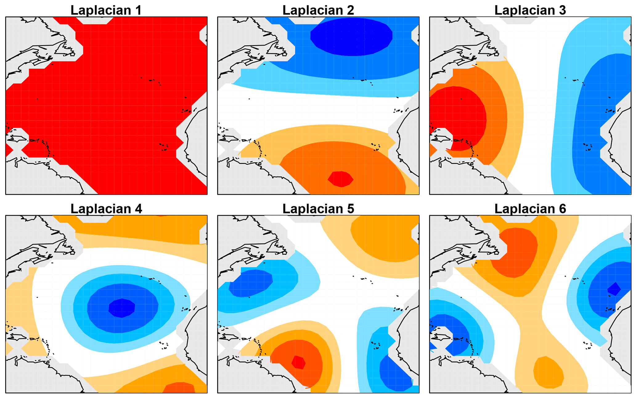
Figure 1Laplacian eigenvectors 1, 2, 3, 4, 5, and 6 over the North Atlantic between the Equator and 60∘ N, where dark red and dark blue indicate extreme positive and negative values, respectively.
For observational data, we use version 5 of the Extended Reconstructed SST data set (ERSSTv5 Huang et al., 2017) and consider the 165-year period 1854–2018. The question arises as to how to extract internal variability from observations. There is considerable debate about the magnitude of forced variability in this region, particularly the contribution due to anthropogenic aerosols (Booth et al., 2012; Zhang et al., 2013). To elaborate, consider the time series for the first Laplacian eigenvector, which we call the AMV index. Figure 2 shows the observed AMV index and the corresponding least-squares fit to second- and ninth-order polynomials in time. The second-order polynomial captures the secular trend toward warmer temperatures but otherwise has weak multidecadal variability. In contrast, the ninth-order polynomial captures both the secular trend and multidecadal variability. There is no consensus as to whether this multidecadal variability is internal or forced. Therefore, to account for either possibility, we analyze two sets of residuals: one in which a second-order polynomial in time is removed from each Laplacian time series and one in which a ninth-order polynomial in time is removed from each Laplacian time series. The residuals are called anomalies, and the anomalies for the first seven Laplacian eigenvectors are shown in Fig. 3. In the case of removing a second-order polynomial, the anomaly time series for Laplacian 1 contains marked multidecadal variability. Comparing such anomalies between observations and control simulations implicitly assumes that this variability is internal variability. In the case of removing a ninth-order polynomial, little to no multidecadal variability is evident in the time series (see the right-hand column of Fig. 3). A 10th- or higher-order polynomial would also remove this multidecadal variability, but following common practice we prefer the lowest possible order. Using anomalies with and without multidecadal variability allows us to draw conclusions while being agnostic about the source of observed multidecadal variability. Note that only Laplacians 1 and 2 are sensitive to this assumption; time series for Laplacians 3 or higher are nearly the same in the two cases.
To be clear, we do not claim that regressing out polynomials perfectly eliminates forced variability. Other methods include subtracting (or regressing out) the global mean temperature (Trenberth and Shea, 2006) or estimating the forced response and using optimal fingerprinting methods to remove forced variability (Bindoff et al., 2013). Each method has its own advantages and disadvantages. We have chosen polynomial fitting because it is simple and the underlying assumptions are clear.
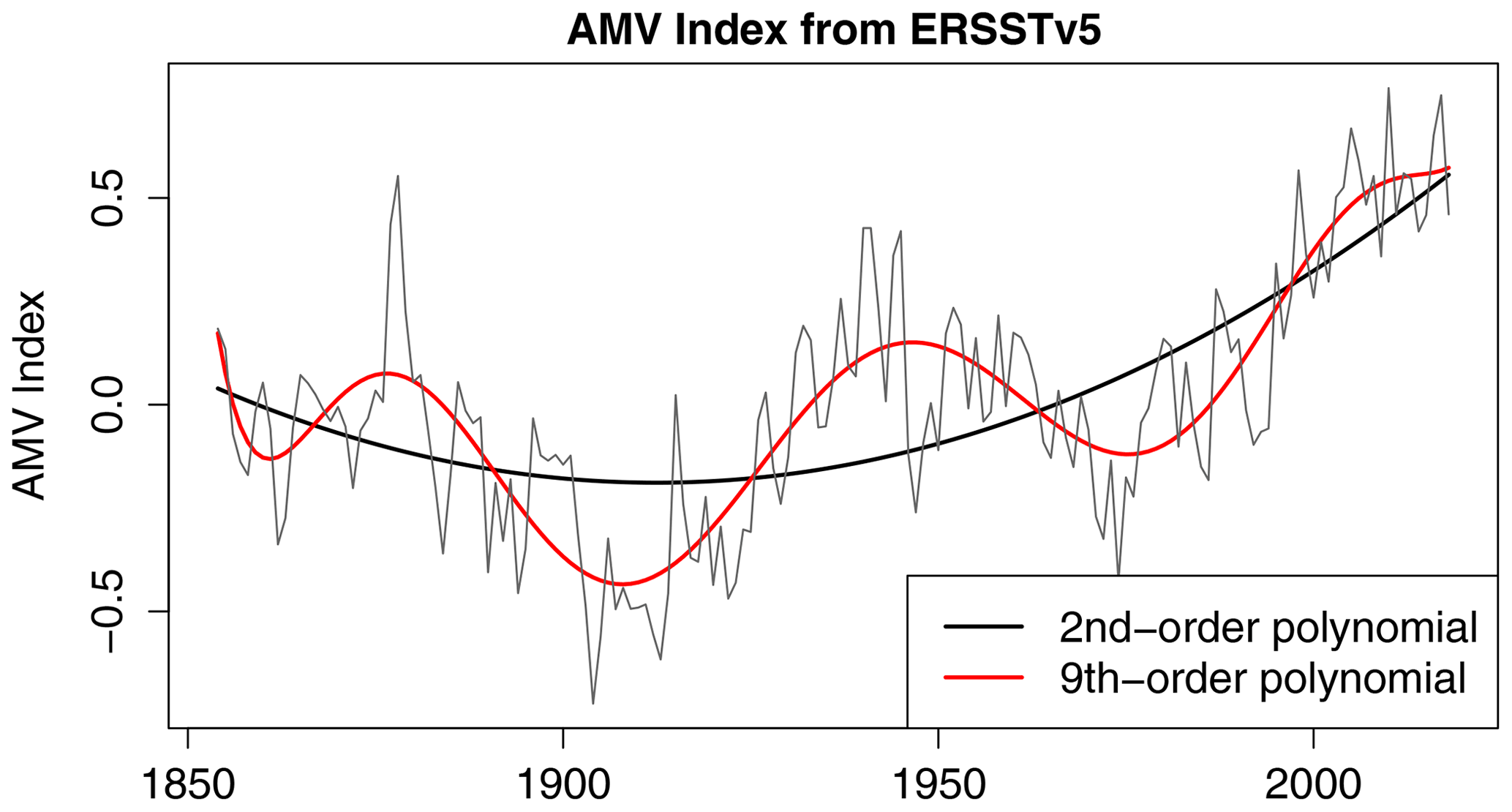
Figure 2AMV index from ERSSTv5 (thin grey) and polynomial fits to second-order (thick black) and ninth-order (red) polynomials.
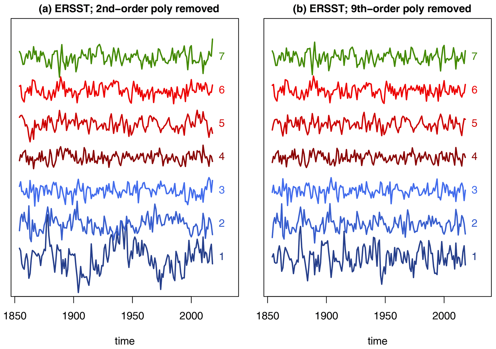
Figure 3Projection of SST anomalies from ERSSTv5 onto the first seven Laplacian eigenvectors of the North Atlantic domain. Panels (a) and (b) show, respectively, anomalies derived by removing second- and ninth-order polynomials in time. The integers on the right end of each time series indicate the Laplacian eigenvector.
Whether observations can be assumed to be stationary is an open question. After all, non-stationary effects may be caused by the changing observational network or by external forcing that is not removed by polynomial fitting (e.g., volcanic eruptions). In addition, some model simulations exhibit surprisingly large changes in variability even without changes in external forcing (Wittenberg, 2009). If a VAR model cannot reproduce such changes, then our test might incorrectly indicate that two realizations from the same dynamical model come from different processes. We investigate these issues in the following way. First, time series of length 165 years are drawn from the control simulations to match the dimensions of the observational time series. Then, each 165-year time series is split in half (82 and 83 years), and time series from the two halves are compared. Our anticipation is that if a time series comes from the same source, then the null hypothesis is true and the method should detect a difference at the expected type-I error rate. This expectation will be checked in the analyses below.
For model data, we use pre-industrial control simulations of SST from phase 5 of the Coupled Model Intercomparison Project (CMIP5 Taylor et al., 2012). Control simulations use forcings that repeat year after year. As a result, interannual variability in control simulations comes from internal dynamical mechanisms. Thus, interannual forced variability is absent in control simulations. Thirty-five CMIP5 models have pre-industrial control simulations of length 165 years or longer.
Model selection
The process of deciding which variables to include in a VAR model is called model selection. Here, model selection consists of choosing the lag p and the number of Laplacian eigenvectors S. While numerous criteria exist for selecting p, there is no standard criterion for selecting S. Note that choosing S is tantamount to choosing both X and Y variables simultaneously, which is a non-standard selection problem. Recently, a criterion for selecting both X and Y variables was proposed by DelSole and Tippett (2021a), called the mutual information criterion (MIC). This criterion is consistent with small-sample-corrected versions of Akaike's information criterion (AIC) for selecting p. In terms of the regression model for Y1 given in Eq. (3), the criterion is
where is the MLE of the covariance matrix of Y1 and
The procedure is to select the subset of X and Y variables that minimizes the MIC. The VAR model selected by this criterion for each CMIP5 model is shown in Table 1. The MIC selects slightly different p and S for each CMIP5 model. However, the difference-in-VAR test requires the same p and S for each VAR model. Therefore, a single compromise model must be chosen. Since the vast majority of selected VAR models are first order, we choose a first-order VAR, which yields a linear inverse model (LIM). Numerous studies have shown that LIMs provide reasonable models of monthly-mean and annual-mean SSTs (Alexander et al., 2008; Vimont, 2012; Zanna, 2012; Newman, 2013; Huddart et al., 2016; Dias et al., 2018). In effect, our method is a difference-in-LIM test. (Incidentally, the MIC provides a criterion for selecting the variables to include in LIMs.) We choose S=7 Laplacian eigenvectors, which is the maximum for any first-order VAR. This choice is more likely to capture important dependency structures than a lower-order VAR model. This choice might also lead to overfitting, but one should remember that the distribution of the deviance statistic does not depend on the actual values of the regression parameters. Consequently, if some regression parameters vanish, indicating that the associated predictors are redundant and can be dropped, the test remains exactly the same as for a model in which all regression parameters are non-zero. The main adverse consequence of including more variables than necessary is a loss of power (i.e., the test is less able to detect a difference when such a difference exists). For our data, this is not a major concern: we consistently find that the test rejects H0 more often as S increases (this will be shown in the Results section). In this study, we are more concerned with capturing important dependency structures than with loss of power, hence our choice to include the maximum number of Laplacian eigenvectors selected by the MIC.
Table 1Models selected by the MIC, based on 82-year time series from each CMIP5 control simulation.

For validity of the significance tests, perhaps the most important assumption is that the residuals of the VAR(p) models form a stationary Gaussian white noise process. Unfortunately, no exact, small-sample test for stationary Gaussian white noise exists, although some approximate tests exist. To check for whiteness of the residuals, we performed the multivariate Ljung–Box test using a maximum lag of 10 years (Lütkepohl, 2005, Sect. 4.4.3). About 20 % of the residual time series were found to have significant non-whiteness. However, this result is sensitive to the choice of maximum lag and to the time period tested, so the interpretation is unclear. After a Bonferroni correction, only one CMIP5 model (CMCC-CMS) had residuals in both time periods that were significantly non-white, which suggests that VAR(1) with S=7 is adequate for our time series.
To be clear, our method can be applied to arbitrary VAR models. Our choice of VAR(1) with S=7 is merely a compromise designed to capture significant large-scale spatial dependencies while also adequately modeling temporal correlations.
Results
The deviance between ERSST 1854–1936 and 82-year segments of pre-industrial control simulations is shown in Fig. 4. Also shown is the deviance between ERSST 1854–1936 and ERSST 1937–2018 (first item on the x axis). The latter deviance falls below the 5 % threshold and hence indicates no significant difference in internal variability between two halves of ERSST, regardless of polynomial fit. This result is consistent with the hypothesis that ERSST is a stationary VAR process after removing either a second- or ninth-order polynomial. Only one CMIP5 model is consistent with ERSST when a second-order polynomial is removed, and only two CMIP5 models are consistent with ERSST when a ninth-order polynomial is removed. We conclude that the vast majority of CMIP5 models generate unrealistic internal variability.
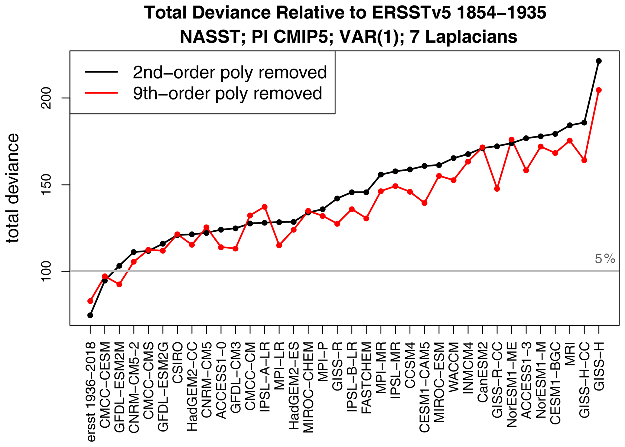
Figure 4Deviance between ERSSTv5 1854–1935 and 82-year segments from 36 CMIP5 pre-industrial control simulations. Also shown is the deviance between ERSSTv5 1854–1935 and ERSSTv5 1937–2018 (first item on the x axis). The black and red curves show, respectively, results after removing a second- and a ninth-order polynomial in time over 1854–2018 before evaluating the deviance. The models have been ordered on the x axis from smallest to largest deviance after removing a second-order polynomial in time.
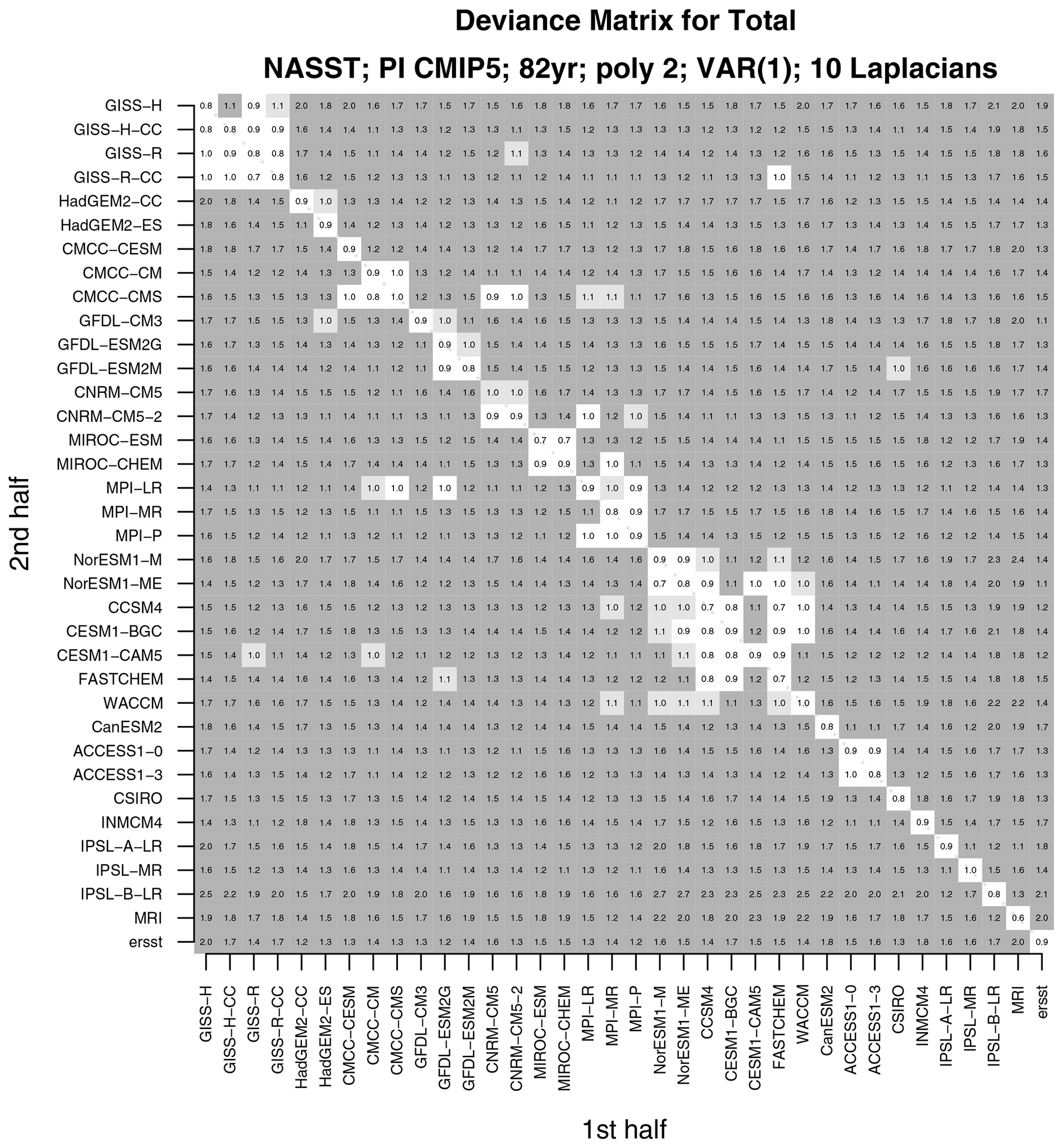
To explore the sensitivity of the above results to the number of Laplacians, deviances based on 10 Laplacian eigenvectors are shown in Fig. 5. In this case, every CMIP5 model differs from ERSST, regardless of which polynomial is removed. More generally, as the number of Laplacian eigenvectors increases, differences between internal variability become easier to detect. Because adding Laplacian eigenvectors corresponds to resolving smaller scales, this pattern means that discrepancies in internal variability become more detectable as smaller-scale spatial structures are taken into account.


Figure 6The deviance between two non-overlapping time series from CMIP5 pre-industrial control simulations and observations. The time series are obtained by extracting a continuous 165-year period, regressing out a second-order polynomial, and then splitting the time series in half (82 and 83 years). For observations, the 165-year period corresponds to 1854–2018. The deviance is divided by the 5 % significance threshold, so values greater than 1 indicate a significant difference in the VAR model. Light and dark grey shadings highlight values greater than the 5 % and 1 % significance thresholds. White spaces indicate insignificant differences between VAR models.
It is instructive to change the reference time series used for comparison. For instance, instead of comparing to ERSST, we compare each time series to time series from the CanESM2 model. The result of comparing every time series from the first half to every time series in the second half is summarized in Fig. 6. The plotted numerical value is the deviance divided by its 5 % critical value. Light and dark grey shadings indicate significant differences at 5 % and 1 %, respectively. Note that the diagonal is unshaded, indicating that the test correctly concludes no difference in the VAR model when time series come from the same CMIP5 model. Some CMIP5 models differ significantly from all other models (e.g., MRI, INMCM4), indicating that these models not only are inconsistent with observations, but are also inconsistent with other CMIP5 models.
Interestingly, models from the same modeling center tend to be indistinguishable from each other (e.g., GISS, NCAR, MPI, CMCC). This result is consistent with previous studies indicating that models developed at the same center show more similarities to each other than to models developed at different centers (Knutti et al., 2013). The deviances for 10 Laplacian vectors are shown in Fig. 7. With more Laplacians comes the ability to detect more differences, so that almost all models are found to differ significantly from each other unless they come from the same center.
An alternative approach to summarizing dissimilarities between models is through dendrograms (Knutti et al., 2013; Izenman, 2013). An example is shown in Fig. 8 and constructed according to the following iterative procedure. First, each multivariate time series is assigned to its own cluster. Next, the pair of time series with the smallest deviance are merged together to form a new cluster. This clustering is indicated by a two-pronged “leaf” whose length equals the deviance. After time series are linked, an “agglomeration” rule is used to measure dissimilarity relative to a cluster. There is no unique choice for the agglomeration rule. We choose a standard one called complete-linkage clustering in which the “distance” between two sets of clusters 𝒜 and ℬ is defined as the maximum deviance between elements of each cluster:
If this distance exceeds the significance threshold, then at least one deviance between elements of the clusters is known to be significant. Then, the smallest distance between any pair of clusters is linked together again. This process repeats until all models have been merged into a single cluster. The x axis shows the distance measure, and the y axis shows the data sources. Each source name occurs twice because two time series are drawn from that source. As can be seen, the shortest leaves are associated with time series from the same source or from models developed at the same center.
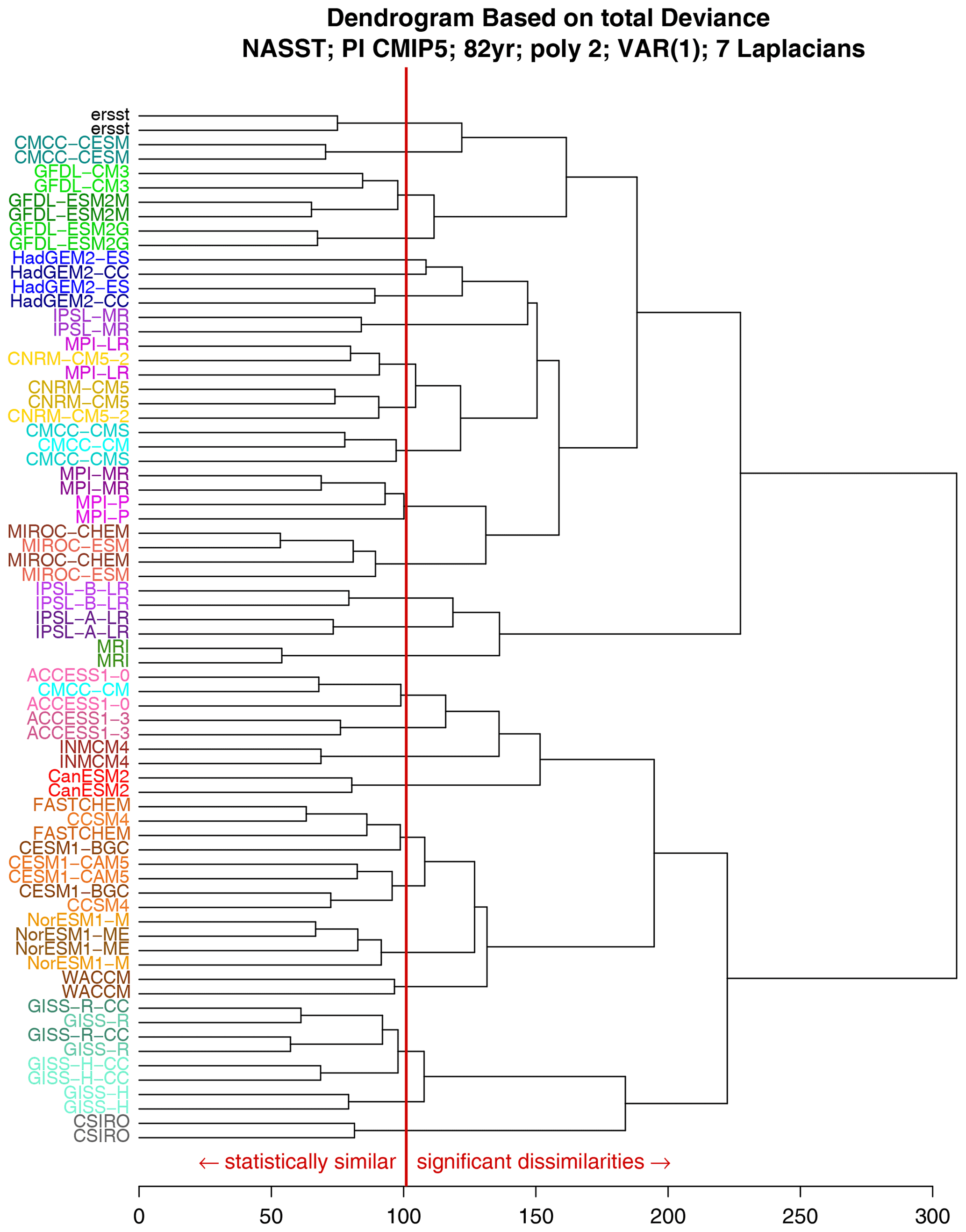
Figure 8Dendrogram derived from the deviance matrix between all pairs of VAR(1) models estimated from the first and second halves of the 1854–2018 period (the specific year is not relevant for pre-industrial control simulations). The clusters are agglomerated according to the complete-linkage clustering, which uses the maximum deviance between elements of each cluster. The VAR models contain seven Laplacian eigenfunctions, and a second-order polynomial in time is removed. The vertical red line shows the 5 % significance threshold for a significance difference in the VAR models.
The broad conclusions drawn from the dendrogram in Fig. 8 are similar to those drawn by Knutti et al. (2013). However, the dendrogram constructed in Knutti et al. (2013) was based on the Kullback–Leibler (KL) divergence. Importantly, KL divergence requires estimation of covariance matrices, but a significance test for this measure was not examined in Knutti et al. (2013). The dendrogram developed here is attractive in that it is based on a rigorous statistical measure of dissimilarity that has a well-defined significance threshold that accounts for sampling variability and dependencies in space and time.
A perennial question is whether models should be weighted equally when making multi-model projections of the future. Such weighting schemes lie outside the scope of this paper, but a related question is whether there exists a relation between a model's past performance and its predictions of the future. To investigate this question, we plot a model's deviance from ERSST against that model's equilibrium climate sensitivity (ECS). ECS is the equilibrium change in annual mean global surface temperature following a doubling of atmospheric CO2 concentration. The result is shown in Fig. 9. The figure also shows a least-squares line fit to the data points. The slope is statistically significant (p=0.011) under the standard assumptions of independent and identically distributed residuals, which of course are dubious for our problem. Nevertheless, the correlation is negative, indicating that models that best simulate the past tend to have larger ECS. Extrapolating to zero deviance yields an ECS of 4.8 ∘C, although the probabilistic meaning (e.g., confidence interval) of this result is unclear.
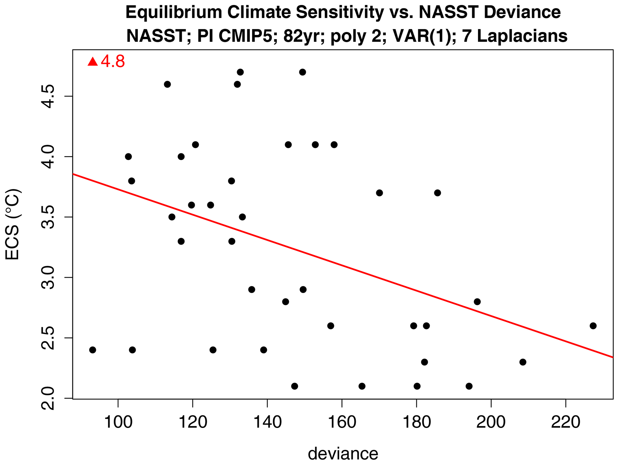
Figure 9Deviance versus equilibrium climate sensitivity of CMIP5 models. The deviance is computed for NASST separately for the first and second halves of the 1854–2018 period, which yields two points per CMIP5 model for a total of 72 points. ECS is derived from Table 9.5 of Flato et al. (2013). The red line shows the least-squares line fit, and the red triangle at the top shows the intercept of the best-fit line.
This paper proposed an approach to deciding whether two multivariate time series come from the same stochastic process. The basic idea is to fit each time series to a vector autoregressive model and then test whether the parameters of the models are equal. The likelihood ratio test for this problem and the associated sampling distributions were derived. This derivation leads to a deviance statistic that measures the difference between VAR processes and can be used to rank models based on their “closeness” to the VAR process inferred from observations. The test accounts for correlations in time and correlations between variables. In the special case of a first-order VAR model, the model is a LIM and the test is effectively a “difference-in-LIM” test.
The test was used to compare internal variability of annual mean North Atlantic SST in CMIP5 models and observations. Internal variability was estimated by removing either a second- or ninth-order polynomial, corresponding to different views about the source of multidecadal variability, as discussed in Sect. 3. Remarkably, almost every CMIP5 model generates internal variability that differs significantly from observations. This conclusion holds regardless of whether a second- or ninth-order polynomial in time is regressed out and therefore is independent of assumptions about whether observed multidecadal NASST variability is forced or internal. Furthermore, the degree of dissimilarity increases when smaller-scale (∼ 2000 km) information is included. Our conclusions are broadly consistent with other studies that have highlighted model inconsistencies; for example, climate models give inconsistent estimates of the magnitude and spatial structure of internal predictability (Branstator et al., 2012). We further showed that time series from the same model or from models from the same modeling center tend to be more similar than time series from models from other centers. These results are consistent with previous claims that the effective number of independent models is smaller than the actual number of models in a multi-model ensemble (Pennell and Reichler, 2011; Knutti et al., 2013). Other studies have shown that models also exhibit significant discrepancies in their forced response. For instance, Zhang et al. (2013) showed that the model response to anthropogenic aerosols exhibits significant inconsistencies with observations, particularly in terms of upper-ocean content, surface salinity, and spatial SST patterns (Zhang et al., 2013). Taken together, these discrepancies imply that, at the present time, climate models do not provide a satisfactory explanation of observed variability in the North Atlantic.
Recently, Mann et al. (2021) argued that there exists no compelling evidence for internal multidecadal oscillations. In particular, oscillations seen in proxies of pre-industrial temperature can be explained as an artifact of volcanic activity that happens to project onto the multidecadal frequency band. Under this hypothesis, variability in NASST is due primarily to external forcing, and removing a ninth-order polynomial would be better at removing forced variability than a second-order polynomial. Nevertheless, even after removing a ninth-order polynomial, our results show that most models are inconsistent with observations.
One limitation of the proposed method is that it assumes that a given time series is adequately modeled as a VAR(p) process. The proposed method could be generalized to VARMA processes. Specifically, maximum likelihood estimates for VARMA models can be used to derive the parameter estimates under H0 and HA, and then the deviance statistic (13) is evaluated. Asymptotically, the parameter estimates have normal distributions, and the distribution of the deviance statistic has a chi-squared distribution with degrees of freedom equal to the difference in the number of parameters between models. The proposed method could also be a starting point for generalizing to cyclostationary or non-stationary processes.
We believe that the proposed method could be valuable for improving climate models. At present, there is no agreed-upon standard for comparing climate models. As a result, different modeling centers use different criteria for assessing their model (Hourdin et al., 2016; Schmidt et al., 2017). The existence of hundreds of metrics leaves ample room for cherry picking. One barrier to forming a consensus is that the available metrics do not (1) account for multiple variables, (2) account for correlations in space and time, and (3) have a rigorous significance test. The deviance statistic satisfies all these conditions. The main remaining barrier would then be to choose a few key climate indices. Although our example uses NASST, any set of relevant climate indices could be used provided they are well modeled by a VAR process. As the number of indices included in the VAR model increases, the sampling variability of the deviance increases (due to the curse of dimensionality), which may make it more difficult to detect discrepancies. Such is the price of a rigorous consistency criterion. However, this pattern need not occur in practice; in our example, inconsistencies became easier to detect as more patterns were included.
Note that using the proposed method to compare observational data sets over the same period would not be straightforward because the two observational data sets would be highly correlated, and therefore the resulting estimates of the noise covariance matrices Γ1 and Γ2 would not be independent, as assumed in the test.
As discussed above, we found that climate model simulations of NASST not only differ from observations, but also between models from different modeling centers. However, this result does not tell us the nature of those differences. A natural question is whether the difference can be attributed to specific parts of the VAR model. Methods for answering this question will be discussed in Part 3 of this series of papers.
An R code for performing the statistical test described in this paper is available at https://github.com/tdelsole/Comparing-Time-Series (DelSole and Tippett, 2021b).
Data are from climate model simulations from phase 5 of the Coupled Model Intercomparison Project (CMIP5), available from https://esgf-node.llnl.gov/projects/cmip5/ (WCRP, 2021).
Both authors participated in the writing and editing of the manuscript. TD performed the numerical calculations.
The contact author has declared that neither they nor their co-author has any competing interests.
The views expressed herein are those of the authors and do not necessarily reflect the views of these agencies.
Publisher’s note: Copernicus Publications remains neutral with regard to jurisdictional claims in published maps and institutional affiliations.
We thank Robert Lund and an anonymous reviewer for comments that led to methodological clarifications and improvements in the presentation of this work. We thank the World Climate Research Programme's Working Group on Coupled Modelling, which is responsible for CMIP, and we thank the climate modeling groups (listed in Table 1 of this paper) for producing and making available their model output.
This research has been supported by the National Oceanic and Atmospheric Administration (grant no. NA20OAR4310401).
This paper was edited by Christopher Paciorek and reviewed by two anonymous referees.
Alexander, M. A., Matrosova, L., Penland, C., Scott, J. D., and Chang, P.: Forecasting Pacific SSTs: Linear Inverse Model Predictions of the PDO, J. Climate, 21, 385–402, https://doi.org/10.1175/2007JCLI1849.1, 2008. a
Allen, M. R. and Tett, S. F. B.: Checking for model consistency in optimal fingerprinting, Clim. Dynam., 15, 419–434, 1999. a
Anderson, T. W.: An Introduction to Multivariate Statistical Analysis, Wiley-Interscience, USA, 1984. a, b
Bindoff, N. L., Stott, P. A., AchutaRao, K. M., Allen, M. R., Gillett, N., Gutzler, D., Hansingo, K., Hegerl, G., Hu, Y., Jain, S., Mokhov, I. I., Overland, J., Perlwitz, J., Webbari, R., and Zhang, X.: Detection and Attribution of Climate Change: From Global to Regional, in: Climate Change 2013: The Physical Science Basis. Contribution of Working Group I to the Fifth Assessment Report of the Intergovernmental Panel on Climate Change, edited by Stocker, T., Qin, D., Plattner, G.-K., Tignor, M., Allen, S., Boschung, J., Nauels, A., Xia, Y., Bex, V., and Midgley, P., chap. 10, 867–952, Cambridge University Press, New York, 2013. a, b
Booth, B. B. B., Dunstone, N. J., Halloran, P. R., Andrews, T., and Bellouin, N.: Aerosols implicated as a prime driver of twentieth-century North Atlantic climate variability, Nature, 484, 228–232, https://doi.org/10.1038/nature10946, 2012. a, b
Box, G. E. P., Jenkins, G. M., and Reinsel, G. C.: Time Series Analysis: Forecasting and Control, 4th Edn., Wiley-Interscience, Hoboken, New Jersey, 2008. a, b, c, d, e
Branstator, G., Teng, H., Meehl, G. A., Kimoto, M., Knight, J. R., Latif, M., and Rosati, A.: Systematic estimates of initial value decadal predictability for six AOGCMs, J. Climate, 25, 1827–1846, 2012. a
Brockwell, P. J. and Davis, R. A.: Time Series: Theory and Metho, 2nd Edn.ds, Springer Verlag, New York, 1991. a, b, c
DelSole, T. and Tippett, M. K.: Laplacian Eigenfunctions for Climate Analysis, J. Climate, 28, 7420–7436, https://doi.org/10.1175/JCLI-D-15-0049.1, 2015. a, b, c
DelSole, T. and Tippett, M. K.: Comparing climate time series – Part 1: Univariate test, Adv. Stat. Clim. Meteorol. Oceanogr., 6, 159–175, https://doi.org/10.5194/ascmo-6-159-2020, 2020. a
DelSole, T. and Tippett, M. K.: A Mutual Information Criterion with Applications to Canonical Correlation Analysis and Graphical Models, Stat, 10, e385, https://doi.org/10.1002/sta4.385, 2021a. a
DelSole, T. and Tippett, M. K.: Software for comparing time series, available at: https://github.com/tdelsole/Comparing-Time-Series, GitHub [code], last access: 29 November 2021b. a
DelSole, T., Tippett, M. K., and Shukla, J.: A significant component of unforced multidecadal variability in the recent acceleration of global warming, J. Climate, 24, 909–926, 2011. a
Dias, D. F., Subramanian, A., Zanna, L., and Miller, A. J.: Remote and local influences in forecasting Pacific SST: a linear inverse model and a multimodel ensemble study, Clim. Dynam., 55, 1–19, 2018. a
Flato, G., Marotzke, J., Abiodun, B., Braconnot, P., Chou, S., Collins, W., Cox, P., Driouech, F., Emori, S., Eyring, V., Forest, C., Gleckler, P., Guilyardi, E., Jakob, C., Kattsov, V., Reason, C., and Rummukainen, M.: Evaluation of Climate Models, in: Climate Change 2013: The Physical Science Basis. Contribution of Working Group I to the Fifth Assessment Report of the Intergovernmental Panel on Climate Change, edited by: Stocker, T., Qin, D., Plattner, G.-K., Tignor, M., Allen, S., Boschung, J., Nauels, A., Xia, Y., Bex, V., and Midgley, P., 741–866, Cambridge University Press, New York, 2013. a
Griffies, S. M. and Bryan, K.: A predictability study of simulated North Atlantic multidecal variability, Clim. Dynam., 13, 459–487, 1997. a
Hourdin, F., Mauritsen, T., Gettelman, A., Golaz, J.-C., Balaji, V., Duan, Q., Folini, D., Ji, D., Klocke, D., Qian, Y., Rauser, F., Rio, C., Tomassini, L., Watanabe, M., and Williamson, D.: The Art and Science of Climate Model Tuning, B. Am. Meteorol. Soc., 98, 589–602, https://doi.org/10.1175/BAMS-D-15-00135.1, 2016. a
Huang, B., Thorne, P. W., Banzon, V. F., Boyer, T., Chepurin, G., Lawrimore, J. H., Menne, M. J., Smith, T. M., Vose, R. S., and Zhang, H.-M.: Extended Reconstructed Sea Surface Temperature, Version 5 (ERSSTv5): Upgrades, Validations, and Intercomparisons, J. Climate, 30, 8179–8205, https://doi.org/10.1175/JCLI-D-16-0836.1, 2017. a
Huddart, B., Subramanian, A., Zanna, L., and Palmer, T.: Seasonal and decadal forecasts of Atlantic Sea surface temperatures using a linear inverse model, Clim. Dynam., 49, 1833–184, https://doi.org/10.1007/s00382-016-3375-1, 2016. a
Izenman, A. J.: Modern Mutivariate Statistical Techniques: Regression, Classification, and Manifold Learning, corrected 2nd Edn., Springer, New York, 2013. a
Keenlyside, N. S., Latif, M., Jungclaus, J., Kornblueh, L., and Roeckner, E.: Advancing decadal-scale climate prediction in the North Atlantic sector, Nature, 453, 84–88, 2008. a
Knutti, R., Masson, D., and Gettelman, A.: Climate model genealogy: Generation CMIP5 and how we got there, Geophys. Res. Lett., 40, 1194–1199, https://doi.org/10.1002/grl.50256, 2013. a, b, c, d, e, f
Kushnir, Y.: Interdecadal variations in the North Atlantic sea surface temperature and associated atmospheric conditions, J. Climate, 7, 141–157, 1994. a
Latif, M., Roeckner, E., Botzet, M., Esch, M., Haak, H., Hagemann, S., Jungclaus, J., Legutke, S., Marsland, S., Mikolajewicz, U., and Mitchell, J.: Reconstrucing, Monitoring, and Predicting Multidecadal-Scale Changes in the North Atlantic Thermohaline Circulation with Sea Surface Temperature, J. Climate, 17, 1605–1614, https://doi.org/10.1175/1520-0442(2004)017<1605:RMAPMC>2.0.CO;2, 2004. a
Latif, M., Collins, M., Pohlmann, H., and Keenlyside, N.: A review of predictability studies of Atlantic sector climate on decadal time scales, J. Climate, 19, 5971–5987, 2006. a
Lütkepohl, H.: New introduction to multiple time series analysis, Spring-Verlag, New York, 2005. a, b
Mann, M. E., Steinman, B. A., Brouillette, D. J., and Miller, S. K.: Multidecadal climate oscillations during the past millennium driven by volcanic forcing, Science, 371, 1014–1019, https://doi.org/10.1126/science.abc5810, 2021. a
Marshall, J., Kushnir, Y., Battisti, D., Chang, P., Czaja, A., Dickson, R., Hurrell, J., McCartney, M., Saravanan, R., and Visbeck, M.: North Atlantic Climate Variability: Phenomena, Impacts, and Mechanisms, Int. J. Climatol., 21, 1863–1898, 2001. a
Newman, M.: An Empirical benchmark for decadal forecasts of global surface temperature anomalies, J. Climate, 26, 5260–5269, 2013. a
Pennell, C. and Reichler, T.: On the Effective Number of Climate Models, J. Climate, 24, 2358–2367, https://doi.org/10.1175/2010JCLI3814.1, 2011. a
Schmidt, G. A., Bader, D., Donner, L. J., Elsaesser, G. S., Golaz, J.-C., Hannay, C., Molod, A., Neale, R. B., and Saha, S.: Practice and philosophy of climate model tuning across six US modeling centers, Geosci. Model Dev., 10, 3207–3223, https://doi.org/10.5194/gmd-10-3207-2017, 2017. a
Taylor, K. E., Stouffer, R. J., and Meehl, G. A.: An Overview of CMIP5 and the Experimental Design, B. Am. Meteorol. Soc., 93, 485–498, 2012. a
Trenberth, K. E. and Shea, D. J.: Atlantic Hurricanes and Natural Variablity in 2005, Geophys. Res. Lett., 33, L12704, https://doi.org/10.1029/2006GL026894, 2006. a
Tung, K.-K. and Zhou, J.: Using data to attribute episodes of warming and cooling in instrumental records, P. Natl. Acad. Sci. USA, 110, 2058–2063, 2013. a
Vimont, D. J.: Analysis of the Atlantic Meridional Mode Using Linear Inverse Modeling: Seasonality and Regional Influences, J. Climate, 25, 1194–1212, https://doi.org/10.1175/JCLI-D-11-00012.1, 2012. a
Washington, B., Seymour, L., Lund, R., and Willett, K.: Simulation of temperature series and small networks from data, Int. J. Climatol., 39, 5104–5123, https://doi.org/10.1002/joc.6129, 2019. a
WCRP: Coupled Model Intercomparison Project 5 (CMIP5), World Climate Research Programme [data set], available at: https://esgf-node.llnl.gov/projects/cmip5/, last access: 1 December 2021. a
Wittenberg, A. T.: Are historical records sufficient to constraint ENSO simulations?, Geophys. Res. Lett., 36, L12702, https://doi.org/10.1029/2009GL038710, 2009. a
Zanna, L.: Forecast skill and predictability of observed North Atlantic sea surface temperatures, J. Climate, 25, 5047–5056, 2012. a
Zhang, R., Delworth, T. L., Sutton, R., Hodson, D. L. R., Dixon, K. W., Held, I. M., Kushnir, Y., Marshall, J., Ming, Y., Msadek, R., Robson, J., Rosati, A. J., Ting, M., and Vecchi, G. A.: Have Aerosols Caused the Observed Atlantic Multidecadal Variability?, J. Atmos. Sci., 70, 1135–1144, https://doi.org/10.1175/JAS-D-12-0331.1, 2013. a, b, c
- Article
(4936 KB) - Full-text XML
realisticdoes not mean that the detailed patterns on a particular day are correct, but rather that the statistics over many years are realistic. Past approaches to answering this question often neglect correlations in space and time. This paper proposes a method for answering this question that accounts for correlations in space and time.