A multi-method framework for global real-time climate attribution

Human-driven climate change has caused a wide range of extreme weather events to become more frequent in recent decades. Although increased and intense periods of extreme weather are expected consequences of anthropogenic climate warming, it remains challenging to rapidly and continuously assess the degree to which human activity alters the probability of specific events. This study introduces a new framework to enable the production and communication of global real-time estimates of how human-driven climate change has changed the likelihood of daily weather events. The framework's multi-method approach implements one model-based and two observation-based methods to provide ensemble attribution estimates with accompanying confidence levels. The framework is designed to be computationally lightweight to allow attributable probability changes to be rapidly calculated using forecasts or the latest observations. The framework is particularly suited for highlighting ordinary weather events that have been altered by human-caused climate change. An example application using daily maximum temperature in Phoenix, AZ, USA, highlights the framework's effectiveness in estimating the attributable human influence on observed daily temperatures (and deriving associated confidence levels). Global analyses show that the framework is capable of producing worldwide complementary observational- and model-based assessments of how human-caused climate change changes the likelihood of daily maximum temperatures. For instance, over 56 % of the Earth's total land area, all three framework methods agree that maximum temperatures greater than the preindustrial 99th percentile have become at least twice as likely in today's human-influenced climate. Additionally, over 52 % of land in the tropics, human-caused climate change is responsible for at least five-fold increases in the likelihood of preindustrial 99th percentile maximum temperatures. By systematically applying this framework to near-term forecasts or daily observations, local attribution analyses can be provided in real time worldwide. These new analyses create opportunities to enhance communication and provide input and/or context for policy, adaptation, human health, and other ecosystem/human system impact studies.

1 Introduction

Many weather and climate events that were rare just a century ago have become more frequent in recent decades (Seneviratne et al., 2021). Though these changing extreme events vary by definition, region, severity, and by their importance for human systems and culture, they all occur on a warming planet that is distinctly and prominently influenced by humans. The observed global mean temperature increase since the preindustrial period is today – and has been for decades (e.g., Hansen et al., 1981) – demonstrably attributable to human activity (Masson-Delmotte et al., 2021). But with the growing influence of human-driven climate change, there is also a growing need to help society recognize how climate change is affecting not only extreme events but also everyday, ordinary weather. Such a recognition would clarify the kinds of conditions that are likely to become more common with climate change and could also help prioritize investments in adaptation.

Extreme event attribution is a relatively new and rapidly growing field within climate science (National Academies of Sciences and Medicine, 2016; Chen et al., 2021, see, e.g., their Cross-Working Group Box: Attribution). Climate attribution studies have shown that a host of weather and climate-related events, including heat waves (Stott et al., 2004), flooding from rainfall and local sea level rise (Van Oldenborgh et al., 2017; Strauss et al., 2021), droughts (Philip et al., 2018b), wildfires (e.g., Abatzoglou and Williams, 2016), intense hurricanes (e.g., Knutson et al., 2019, and references therein), and “compound events” (i.e., multiple climate hazards that combine to drive environmental or societal impacts, e.g., Zscheischler et al., 2018) have been influenced by anthropogenic climate change since the preindustrial period. Beyond attributing physical changes to human influences on the climate system, there is a growing and vital body of literature now attributing heat-related illness (Vicedo-Cabrera et al., 2021; Mitchell, 2021; Perkins-Kirkpatrick et al., 2022) and economic damages from extreme weather (Strauss et al., 2021).

The concept of “rapid attribution” (National Academies of Sciences and Medicine, 2016) – i.e., the assessment and delivery of quantitative attribution analyses shortly after an extreme event – has been developed to attribute specific events, including regional drought (Otto et al., 2018), extreme heat (Kew et al., 2019; Philip et al., 2021), and flooding from extreme rainfall (Van Der Wiel et al., 2017; Philip et al., 2018a). Pioneering projects such as World Weather Attribution initiative (WWA; https://www.worldweatherattribution.org/, last access: 2 June 2022) have made considerable progress in reducing the time between an event and the release of an attribution assessment. These assessments require a ready and available research team working rapidly after an event occurs. As of 2021, “rapidly” still means attribution information is often not available for days to months after an event (e.g., Philip et al., 2021). This delay constrains the ability of media and policymakers to discuss the links between weather and climate. High-quality and hands-on attribution approaches also require someone to select the events that will be studied. Consequently, rapid attribution research is most often applied to the most extreme events in the developed world rather than lesser-known (but nonetheless attributable) events that are occurring across the planet (Sippel et al., 2020; Callaghan et al., 2021). But climate change is influencing the odds of day-to-day observed weather events as well. Our study focuses on attributing human-caused climate influences on these relatively more common occurrences.

We have developed a global framework to quantify whether and how much human-caused climate change has changed the likelihood of daily local weather events from the preindustrial climate to today. Our goal is to enable daily attribution assessments that support and frame climate change communication for a broad range of users and audiences from the very start of an event. The approach is designed to be (1) rigorously based on existing principles and methods in attribution science (as described primarily in National Academies of Sciences and Medicine, 2016, and van Oldenborgh et al., 2021), (2) adaptable to a range of environmental state variables that are sensitive to global mean temperature changes, and (3) computationally tractable, enabling same-day local event attribution worldwide in support of daily operational deployment. Our system can quickly calculate the probabilities of an observation or forecast in both modern and preindustrial/counterfactual climates. Climate attribution remains underexplored. Historically, there are substantially fewer attribution events studied than attributable events that have occurred, particularly in the developing world (Otto et al., 2020). The global scope of our framework's design enables the production and dissemination of daily attribution estimates in these parts of the world, in addition to the better-studied European and North American regions.

The framework is intended to complement existing attribution approaches (i.e., WWA rapid attribution). Multiple methods are employed to perform attribution calculations. The framework also quantifies uncertainty for each method, either directly through resampling or indirectly by taking advantage of the method's underlying data structure (e.g., intermodel uncertainties characterized by an ensemble). Synthesis across results from multiple methods then informs a final attribution assessment.

This study is meant as an illustrative introduction to this new real-time-capable attribution system. Section 2 describes the framework methodology, exploring the assumptions, statistics, uncertainty quantification, and flow of the approach. It also details the simulated and observed maximum daily temperatures we use to demonstrate the attribution framework. Real-world applications of our system to a particular place and time (July 2016, Phoenix, AZ, USA), a set of point locations from each continent, and a sample broad global analysis, are presented in Sect. 3. Section 4 concludes with a discussion of the framework's value, limitations, opportunities for improvement, and potential future applications.

2 Framework development

2.1 Overview

We construct a methodological framework to make comprehensive worldwide assessments of the role of human-driven climate change in local daily weather events, at predefined spatial scales and for predefined variables, and draw inspiration and guidance from rapid and traditional attribution studies. This section provides a high-level overview of the attribution framework; a glossary of key study terms is provided in the Supplement (Table S3).

The approach streamlines existing, mature techniques described in the National Academies of Sciences (NAS) report on the “Attribution of Extreme Weather Events in the Context of Climate Change” (National Academies of Sciences and Medicine, 2016) and in procedures outlined by the WWA collaboration (van Oldenborgh et al., 2021). Specifically, we frame our attribution analyses around objective selection criteria defining events using either percentile or absolute value thresholds. This framing allows us to quantify (and even discover) attribution estimates across a full range of less extreme/less well-known events that have been made more extreme by human activity and cause considerable impacts on human systems (e.g., Wang et al., 2021). Attribution estimates are defined with a hazard-based approach that focuses on how the probability of event occurrence responds to human-caused climate change (this is called a “risk-based approach” in Jézéquel et al., 2018)¹.

We quantify attribution estimates by contrasting event likelihoods from an observed or modeled “forced” distribution (which has been influenced by human activity since the late 19th century) of a single Earth system state variable of interest (temperature, soil moisture, humidity, etc.) to a defined “counterfactual” distribution of that variable (which is assumed to have not been significantly influenced by human activity, e.g., Otto, 2017). To arrive at these forced and counterfactual distributions, our system uses three complementary methods – two that use observations and a third that uses climate model simulations – described in more detail in Sect. 2.3. Briefly, the three methods are as follows:

• Method no. 1 – observation-based median-scaling method. Forced and counterfactual distributions are found by scaling the observed climatological distributions of the state variable, based on the relationship between their monthly medians and annual global mean surface temperature (GMST).

• Method no. 2 – observation-based quantile-scaling method. Forced and counterfactual distributions are found by scaling and aggregating individual distributions of monthly calculated quantiles from the state variable's observed climatology. Scaling is based on the individual relationships between each monthly quantile and annual GMST.

• Method no. 3 – model-based attribution method. Historical plus projected and natural distributions of the state variable are drawn from an ensemble of bias-adjusted climate models to form forced and counterfactual distributions, respectively.

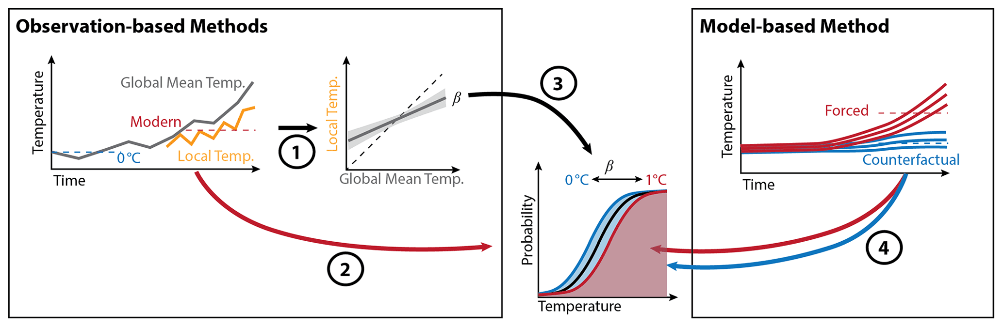
Figure 1 Diagram of this study's multi-method approach to quantifying local climate attribution estimates. The two observation-based methods begin by (1) relating the local temperature (orange) to GMST (gray) to obtain β, which is the change in local mean temperature with a change in GMST. This includes an error estimate from the linear regression. (2) Observational data are used to characterize a climatological (1985–2015) distribution of temperatures (black curve). (3) Then, the median-scaling method uses β to shift the climatological distribution backward to a preindustrial counterfactual climate (blue curve and shading) and either backward or (typically) forward to a forced distribution of temperatures contemporary with the events being attributed (red curve and shading). Shifts based on GMST are assumed to be completely driven by historical, human-emitted greenhouse gases. The quantile-scaling method uses the same procedure, but models separate β values across 30 specified distribution quantiles. The model-based method uses climate model simulations to characterize the local temperature under natural forcing (blue lines) or in a climate forced by human-emitted greenhouse gases (red lines). (4) The forced and counterfactual distributions of temperatures used to quantify attribution estimates are then inferred directly from the three methods.

Each method offers different lines of evidence for the extent to which changes in a state variable are attributable to anthropogenic climate change (consistent with the approach of several modern attribution studies, e.g., Eden et al., 2016; Philip et al., 2020; van Oldenborgh et al., 2021). Throughout this study, we use the change in GMST as an indicator of global warming due to anthropogenic greenhouse gas emissions (as described in Sect. 2.3.1).

The observation-based methods begin by characterizing how the variable of interest (in this study we consider the daily maximum temperature) changes as a function of GMST (Fig. 1; arrow 1). GMST is first aligned relative to a preindustrial reference period (1850–1900, as defined by the Intergovernmental Panel on Climate Change; Masson-Delmotte et al., 2018; Sect. 2.2.1) approximating the climate system before significant human influence on global surface temperatures. We then use the relationship between the variable and GMST to translate an observed climatological distribution (Fig. 1, arrow 2) into two different distributions representing the forced and counterfactual climates (Appendix B), respectively. In our case, we contrast a counterfactual representing a preindustrial past climate with the current human-driven climate that is globally about 1.1 ^∘C warmer (Fig. 1; arrow 3; Fig. S1 in the Supplement). We note that this method could, in principle, be extended to consider the attribution of future warming outcomes (e.g., with a target such as the well-known +1.5 ^∘C); this approach has been used with models in Seneviratne et al. (2016), applied in recent WWA studies, and was explicitly discussed in Otto et al. (2018). Because our study goal is to calculate attribution estimates for current daily events, we focus here on historical human-induced warming. The median-scaling observation-based method (method no. 1 above) uses the relationship between GMST and the local state variable's median to shift the distributions. The more complex quantile-scaling method (method no. 2 above) allows state variable quantiles to shift at different rates with GMST, enabling the distribution to stretch or compress as it is translated. The third model-based method contrasts the state variable distribution in greenhouse-gas-forced climate model simulations with a counterfactual distribution derived from the unforced natural model runs (Fig. 1; arrow 4). Note that while these methods are not fully independent, they offer distinct perspectives and assumptions to determine the historical and counterfactual distributions used in attribution calculations.

The state variable we use to illustrate the application of the new framework is the daily maximum temperature (T_max). We focus on T_max for four key reasons. First, there is ample evidence that attributable climate change has already affected historical daily T_max (e.g., Seneviratne et al., 2021). Second, the connections between human-caused climate change and T_max, idealized by a linear shift in temperature distributions as the climate system warms, are relatively straightforward to explore and explain with thermodynamic arguments (Trenberth et al., 2015). Third, extreme heat is a major driver of human health impacts, and these effects are expected to worsen in the near- and long-term as the climate warms (Ranasinghe et al., 2021, and references therein). Accordingly, it is advantageous to quantify and communicate attribution estimates of extreme heat on short timescales for the public and decision-makers. Finally, T_max is a fundamental climate variable with a long observational history, and temperature trends are generally well-represented by global climate model simulations (e.g., Zwiers et al., 2011; Sillmann et al., 2013; Tebaldi and Wehner, 2018)². Although substantial regional uncertainties from internal climate fluctuations may still affect regional trends and hamper the climate signal's emergence (especially at higher latitudes, e.g., Deser et al., 2012), ongoing attributable climate warming should progressively overwhelm this natural variability. T_max will thus become a better simulated state variable for attribution analyses over time. In cases or regions where historical climate-modeled temperature trends are inconsistent with observations, our framework's incorporation of observation-based estimates safeguards against overconfidence (or blind acceptance of model results) when making attribution assessments (Sect. 2.4).

2.2 Data

2.2.1 Observations

Observed T_max data are drawn from the Berkeley Earth daily land gridded product (Muller et al., 2013; Rohde et al., 2013) over 1880–2017. T_max data are provided at 1×1^∘ native resolution over all land locations and are regridded to N96 spatial resolution (1.875×1.25^∘) to compare with model simulations. We remove leap days to directly compare with 365 d model simulations. Though the Berkeley Earth dataset nominally has data since 1850, the first available year of analysis varies by location; global land coverage (excluding Antarctica) is fully maintained starting in 1955 (Fig. S2). Because GMST trends can now be robustly detected since 1980 (with an extremely likely attributable fraction of ∼85 %, as shown by Sippel et al., 2021), we consider this ≥65-year period a sufficient basis for analyzing attributable changes in T_max probabilities.

We take the monthly GMST time series from the Met Office Hadley Centre/Climatic Research Unit Temperature data set, version 5 (HadCRUT5; Morice et al., 2021). HadCRUT5 GMST anomalies are calculated relative to 1850–1900, i.e., the IPCC reference period for defining global warming with respect to preindustrial conditions (e.g., Masson-Delmotte et al., 2018), enabling the straightforward attribution of human-driven GMST changes (Sect. 2.3) and preserving the temporal reference between observations and climate models (Sect. 2.2.2). We smooth the GMST anomaly time series (hereafter, annual GMST) with a 36-month boxcar filter to dampen noise from internal variability in the climate system (Fig. S1). Note that we recomputed our analysis through 2016 with the Cowtan and Way (2014) GMST dataset and found that our results are qualitatively insensitive to this choice.

2.2.2 Models and bias adjustment

Daily surface maximum temperatures and mean temperatures are drawn from the global climate model output of the Coupled Model Intercomparison Project phase 5 (CMIP5; Taylor et al., 2012) over the following three experiments: a historical simulation including both natural and human forcing over 1860–2005 (historical), a historical simulation with only natural forcing over 1860–2005 (historicalNat, hereafter referred to as the natural experiment), and a future high emissions forcing scenario (rcp85; Riahi et al., 2011). All CMIP5 data are regridded to a common global N96 grid (shared with regridded observations; see above) and GMST anomalies are shifted uniformly over time to set each model's baseline average GMST anomaly to 0 ^∘C across the IPCC 1850–1900 preindustrial reference period (to mirror observed annual GMST). Historical and RCP8.5 experiments are concatenated to form an uninterrupted time series of T_max and GMST for each model over 1860–2050 (hereafter, historical plus projected), which are used to define the forced distributions in attribution analyses (see below). We use 35 simulations in total. There are 11 models with paired historical plus projected and natural forcing experiments and 13 models with a historical plus projected forcing experiment only (i.e., simulations without a paired natural experiment; Table S1).

Before model simulations can be used in attribution analyses – especially when evaluating the probabilities of specific absolute temperatures – they must be bias adjusted. We apply a trend-preserving bias adjustment method developed by Lange (2019). It is a modified parametric quantile-mapping approach that is designed to adjust biases while preserving trends across the full range of a distribution's quantiles. Because we are concerned with a single variable of interest in this study, T_max (so that our application does not require preserving diurnal temperature range or skew; e.g., Piani et al., 2010), we may directly apply the methodology for bias adjusting near-surface air temperature (tas) to bias adjust T_max. The method, detailed in Appendix A, produces bias-adjusted historical plus projected and natural simulated time series of T_max. These time series are used to define the modeled forced and counterfactual distributions for attribution analyses, as described in Sect. 2.3.2.

2.3 Methods

2.3.1 Observation-based attribution analysis

The observation-based methods first determine the relationship between the state variable of interest and GMST (arrow 1 in Fig. 1). This involves a key assumption that 100 % of the observed GMST mean change since the preindustrial period is attributable to factors from human-caused climate change (Fig. S1). Following directly from the IPCC AR6, median estimates of human-caused warming and GMST changes since 1850 are approximately the same (1.07 and 1.06 ^∘C, respectively; Eyring et al., 2021). The assumption of 100 % attributable warming may also be conservative, i.e., in the absence of human-induced warming, modeling and paleoclimate evidence suggests that GMST might have exhibited a cooling trend over the last 170 years, offering a potential alternative counterfactual (e.g., Jones et al., 2012; Kaufman et al., 2020).

In the median-scaling method, a set of scale factors, β (in units of ^∘C [T_max] per ^∘C [GMST]; Appendix B), are calculated separately for each month from the regression between a yearly time series of each month's median T_max (derived from each individual month's daily data), $T_{\max }{,}_{q_{\mathrm{50}}}$, and the smoothed time series of annual GMST; the regression is performed over all years of available T_max data at each individual grid point (Fig. S2), resulting in 12 median-derived monthly scale factors per location (Fig. S3).

The quantile-scaling method mirrors the median-scaling method, except that monthly scale factors are calculated and distributions are scaled over a set of quantiles derived from the daily data. We find temperatures associated with each of 30 quantiles – chosen to be analogous to the number of days in an average month – roughly equally spaced between 0.01 and 0.99 (the full set of quantiles is in Sect. S1 in the Supplement), resulting in 30 annual quantile time series of maximum temperature, $T_{\max }{,}_{q_i}$, per location and month, and spanning the range of available years of data at that individual grid point. Next, scale factors are calculated by regressing each quantile time series against annual GMST, producing $\mathrm{12}\times \mathrm{30}=\mathrm{360}$ total scale factors per location (Fig. S4).

In each method, as described in Appendix B, the resulting scale factors for a given month and location are used to translate a monthly climatological distribution according to the difference between the climatological mean GMST and a target GMST. The target GMST for the forced distribution is 1.07 ^∘C, equal to the contemporary (2010–2019) mean global warming relative to the 1850–1900 preindustrial reference period (Fig. S1; Masson-Delmotte et al., 2021). The target temperature for the counterfactual distribution, representing a preindustrial period without significant attributable human influence on GMST, is the 1885–1915 GMST mean (1.13 ^∘C cooler than the contemporary forced distribution; Fig. S1). For the mean-scaling method, daily data are shifted based on the month in which they are recorded. For the quantile method, each quantile time series is shifted to a forced or counterfactual distribution by multiplying that quantile's monthly scale factor by the target's GMST mean difference from the climatology. The resulting temperatures (30 per month, i.e., one for each quantile) are pooled across the quantiles to form translated forced and counterfactual temperature distributions.

Median- and quantile-scaling methods have different assumptions and tradeoffs. Median-scaling follows a traditional perspective of climate change's influence on temperature in that GMST warming will cause a linear shift in the state variable distribution while its shape remains fixed (e.g., Hansen et al., 1988, Rahmstorf and Coumou, 2011, Hansen et al., 2012, and National Academies of Sciences and Medicine, 2016 (their Fig. 1.1)). Median-scaling thus explicitly assumes that shifts correlated with human-driven GMST changes are trend stationary; this approach is elegant (because changes in tail probabilities are easily interpretable) and produces stable signal-to-noise estimates, but it may be too simplistic under some situations. For example, it could fail in humid maritime climates where an upper limit on daily T_max is set by local convection (e.g., Emanuel et al., 1994; Williams et al., 2009; Sherwood and Huber, 2010, note that this bound shifts with sea surface temperature warming), or in the midlatitudes where soil–moisture feedbacks can drive increases in temperature variance with warming (e.g., Vogel et al., 2017, see Sect. 3.1.1). In contrast, the quantile-scaling method enables the implicit quantification of these features by assuming that the rate of the variance shift in the local temperature distribution (as determined by the collective set of linear scalings between each individual quantile and GMST at a given location and month) is fixed. This approach models a more physically consistent and historically realistic shift of the state variable's distribution in exchange for increased computational and interpretational complexity. Furthermore, because there are fewer historical observations providing information in the distribution tails, we would expect each individual quantile in the tail to have lower precision (and potentially lower accuracy) than those estimated from the central part of the distribution, possibly resulting in noisier attribution estimates. We therefore use both median-scaling and quantile-scaling estimates in this study to strike a balance between historical realism and robustness. Note that the temperature values associated with each quantile (defined from the climatological distribution) could cross each other during the scaling process. Since we treat each set of 30 quantiles as a monthly distribution for attribution analysis (from which we calculate a new set of quantiles during assessment; Sect. 2.4), the results from our method are unaffected by such crossings.

For our demonstration in this study, we use the median- and quantile-scaling methods to translate 31-year climatological distributions of observed daily T_max values from 1985–2015 (arrow 2 in Fig. 1) into a set of forced and counterfactual distributions for use in attribution analyses (arrow 3 in Fig. 1). Each monthly climatological distribution (containing 31 years and 28→31 d, composing a total of 868→961 individual temperatures) is translated separately according to their monthly scale factors. After scaling, the resulting forced and counterfactual distributions are composed of 31 years of daily (or quantile) T_max values. A 31-year time interval is advantageous because it is closely tied to the classical definition of climate (e.g., the 30-year intervals defined by Organization, 2017) and because it balances two competing interests, namely the relevance of the climate mean state for recently observed events versus the statistical robustness of results. While a shorter averaging window (e.g., 5 years) might more precisely describe the warming that is being experienced during a given event, the observed changes will have broader uncertainty due to internal variability. Likewise, a longer integration window (e.g., 50 years) could potentially have unrepresentative and outdated warming relative to recent extreme events, which would underestimate the modern attributable human influence.

In each method, we implement uncertainty analyses to produce distributions of attribution estimates. This allows the attribution framework to provide not only median attribution estimates but also confidence intervals quantifying the robustness of attribution estimates and enabling inter-method statistical comparisons (Sect. 2.4). Spatially resolved uncertainty analyses are an important component in the anticipated operational deployment of this system because they enable communication on the degree of confidence associated with each individual attribution estimate. Note that our analysis does not quantify structural/intrinsic uncertainties in our methods (such as the assumption of linearity, which may not correctly represent every historical relationship between T_max and GMST; Chen et al., 2019). Potential improvements addressing these are discussed in Sect. 4.

Trends and correlations in local T_max and GMST – forming the basis of these observational-based approaches – may be sensitive to local internal variability. For instance, a single particularly warm year near the end of the record (or cold year at the beginning of the record) could increase both the GMST and T_max trends, resulting in a higher scale factor and potentially overestimated attribution estimates. Likewise, there are regression uncertainties between GMST and the state variable arising from weather noise. Accordingly, we use a bootstrapping technique (e.g., Efron and Gong, 1983) to quantify the scale factor uncertainty from variability in both observation-based methods. Using the median-scaling approach as an example, the Monte Carlo resampling recipe is as follows:

1. At each month and location, find the median time series (as described above), $T_{\max }{,}_{q_{\mathrm{50}}}=(T_{\mathrm{1}},T_{\mathrm{2}},\mathrm{\dots },T_i,\mathrm{\dots },T_{n-\mathrm{1}},T_n)$, where n is the total number of years in the annual time series.

2. Where N is the number of samples to collect, repeat N times as follows:

   1. For each i^th year, randomly draw a year k with equal probability from a 3-year window³ around i, i.e., from $U\mathit{\{}i-\mathrm{1},i,i+\mathrm{1}\mathit{\}}$. End points, i=1 and i=n, are resampled identically to their neighboring year (i.e., i=2 and $i=n-\mathrm{1}$). Then, T_i is replaced with T_k in the time series.

   2. Compute the associated scale factor by regressing the resulting time series against annual GMST (Appendix B).

3. Pool each of the N scale factors to form a distribution from which we derive scale factor confidence intervals.

Resampled quantile-scaling distributions are found with the same sequence, replacing the median annual time series with each quantile annual time series, $T_{\max }{,}_{q_i}$. In this study, we take N=1000. The resulting scale factor confidence intervals are carried through attribution implementation to produce confidence intervals of attribution estimates, which in turn inform the final assessments of attribution (Sect. 2.4).

2.3.2 Model-based attribution

The model-based method defines the forced and counterfactual distributions (arrow 4 in Fig. 1) from the ensemble of bias-adjusted climate model simulations. We first extract the final 31-year period of the natural CMIP5 runs (i.e., the 1975–2005 climate which evolved in the absence of human-forcing by greenhouse gas emissions). After bias-adjustment (Sect. 2.2.2; Appendix A), T_max distributions from each of the 11 natural simulations are pooled into a single distribution. This pooled distribution, composed (on average) of ∼10 400 T_max values at each location and in each month, defines the final model-based counterfactual distribution. Note that we use pooling to define the counterfactual to make use of the full ensemble of forced distributions (24 CMIP5 models in total) following a technique from recent attribution work (Strauss et al., 2021). An alternative is to define individual counterfactual distributions from each natural simulation (which are paired to a historical plus projected simulation; Table S1). Although this would considerably decrease the sample size (from 24 forced distributions to 11 model pairs), it could more accurately portray model attribution results.

Next, we find the calendar year when each model's historical plus projected 31-year centered-running-mean of GMST exceeds 1.07 ^∘C (relative to the preindustrial reference period). This year is taken to be the midpoint of a 31-year time series making up that model's defined simulated forced distribution of T_max at each location (31-year intervals for each model are provided in Table S1; cf. Fig. S1). An uncertainty analysis to assess the statistical robustness of model-based attribution considers the ensemble spread among these forced distributions.

2.4 Implementation and assessment

Following a hazard-based framing, the attribution framework uses coupled changes in GMST and maximum temperature exceedance probabilities to determine the extent and confidence level of attributable human-influence on daily temperature events. At a given absolute temperature or quantile, the ratio of exceedance probabilities between the forced and counterfactual distributions provides an estimate of how that quantile or temperature has shifted because of human-caused climate change. We quantify this shift using the (exceedance) probability ratio (e.g., Fischer and Knutti, 2015; Sippel et al., 2016; Otto et al., 2018; Philip et al., 2020; van Oldenborgh et al., 2021), $\mathrm{PR}\equiv \frac{p_{\mathrm{forced}}}{p_{\mathrm{cf}}}$, where p_forced is the probability of exceeding a specific temperature threshold (in the context of a given temporal unit of analysis, e.g., monthly, seasonal, or annual) from the forced distribution, and p_cf is the corresponding probability of exceedance from the counterfactual distribution.

At each global location and for each of the forced and counterfactual distributions, these probabilities can be calculated by integrating daily exceedances of an absolute temperature threshold. We either prescribe this temperature directly or infer it from a prescribed quantile. Integration is performed using the counterfactual climatology of each distribution set (i.e., via median-scaling, quantile-scaling, and modeling methods) and can be done in the context of monthly, seasonal, and annual units of analysis. For each given threshold and context, we calculate PR over the 31 years of the paired forced/counterfactual distributions. Because we seek the climatological PR of any given year (rather than a specific year), our final attribution estimate for each method is given by the mean over the 31 individual-year PR values. We fully describe our calculations that quantify PR based on discrete exceedance counts in Appendix C.

PR uncertainties are determined by calculating PR values using the full distributions of either resampled scale factors and their paired forced/counterfactual distributions (observation-based methods) or each individual forced climate model distribution against the pooled counterfactual distribution (model-based method). To determine the statistical significance of attribution from the resulting PR distributions, we compare 95 % confidence intervals of each method against a null hypothesis that exceedance probabilities should be the same between the forced and counterfactual climates, i.e., $H_{\mathrm{0}}:\mathrm{PR}=\mathrm{1}$. In the case of model-based estimates, attribution is determined to be statistically significant if 23 out of the 24 simulated PR>1 at 96 % confidence with a one-sided interval (the same logic can also be applied to test PR<1).

Discrete exceedance count calculations (Appendix C) cannot appropriately quantify probability changes in the extreme tails of the 31-year forced and counterfactual temperature distributions. This is because there are too few temperature observations exceeding⁴ far-tail quantiles to accurately represent the unknown true underlying distribution of extreme values. Extreme value theory is typically applied in these cases to more accurately represent tail probabilities (Coles, 2001, see below). To account for this limitation in our approach, we define an upper-tail “critical quantile” as being the point where the number observations in the climatological distribution that are expected to exceed the quantile equals one per year (within the unit of analysis). The value of the critical quantile follows directly from the definition of the quantile (Table S2; Appendix C). Upper-tail critical quantiles for the monthly, seasonal, and annual units of analysis are 0.967, 0.989, and 0.997, respectively. For any distribution being analyzed, an absolute temperature threshold may be found using the critical quantile. Herein we do not calculate PR values at temperatures that are higher than the absolute temperature thresholds derived from the climatology (see Sect. 3). Instead, we assert that PR values calculated at the critical quantile are a lower bound on PRs associated with T_max values above the critical quantile; this is a conservative choice, assuming that PR values grow monotonically with temperature increases (Sect. 3).

Attribution of temperatures above the critical quantile could be performed using generalized extreme value distributions, as is often done in traditional attribution studies of extreme events (e.g., Huang et al., 2016; Diffenbaugh et al., 2017; Van Oldenborgh et al., 2017; Otto et al., 2018; Wehner et al., 2018; Kew et al., 2019; Philip et al., 2021, and many others). However, events which require the use of extreme value theory could benefit from more in-depth study than our lightweight hazard-based approach affords. Our method provides a way of making an initial statement about climate change's influence on these events and objectively identifying events that might warrant deeper analysis. We therefore omit extreme value attribution estimates in our current implementation of the framework in favor of the computational efficiency and communication expediency supplied by lower bound estimates from critical quantiles.

3 Results

We use three examples to illustrate the temporal and spatial performance of our attribution framework. We first present an example from Phoenix, AZ, USA, that shows how our three methods work in practice over a month of daily data and how their results can be combined to make a final attribution assessment. We then extend our case study to include attribution estimates at various locations around the world on a single day. Finally, we consider the global spatial fingerprint of human-caused climate change by looking at worldwide probability ratios for each location's 99th percentile maximum temperature.

3.1 Real-world application: results from Phoenix, AZ, USA

As an example application of our real-time attribution system, we use each method to assess the attribution of Phoenix T_max in July 2016. Phoenix has recently experienced deadly extreme heat events (as has much of the western United States, e.g., June 2021; https://www.climate.gov/news-features/event-tracker/record-breaking-june-2021-heatwave-impacts-us-west, last access: 2 June 2022), but how attributable are Phoenix days with less extreme maximum temperatures? To briefly explore this question, we examine the month of July 2016 because it exhibits a relatively calm period of warm weather, exemplifying a set of “lesser extreme” moderately high temperatures that are nevertheless made more frequent by climate change. Daily July 2016 T_max observations are taken from the Berkeley Earth dataset at the grid point containing Phoenix (33.75^∘ N, 112.5^∘ W; the city center is approximately 52 km from the containing grid cell's center). Note that we are using a coarse analysis grid to illustrate the attribution framework; gridded data could be downscaled and combined with point-based (e.g., station) data to produce more accurate estimates at a specific point (see the discussion in Sect. 4).

For each daily observation, we use each of the three framework methods to calculate probability ratios from July forced and counterfactual distributions (i.e., over the July monthly unit of analysis). Daily PR values illustrate how the probability of meeting or exceeding Phoenix's daily observed T_max has changed across the month of July because of human-caused climate change.

3.1.1 Seasonal cycle analysis

We first analyze Phoenix PR values calculated from each method over each monthly unit of analysis (January through December) at the 95th percentile of each counterfactual distribution. Seasonal cycles of PR medians and 95 % confidence intervals (from the observation-based method PR distributions) and individual-model PRs are plotted in Fig. 2. The influence of human-driven climate change is clear, robust, and strongly attributable across the upper tails of monthly Phoenix T_max. Out of 36 total estimates (12 months and 3 methods), 33 have PR>1.0 and are statistically significant at 95 % confidence. The rare insignificant values – a single observation-based PR (December; median scaling) and two model-based estimates totaling five individual model runs (in February and March) – fall in winter months.

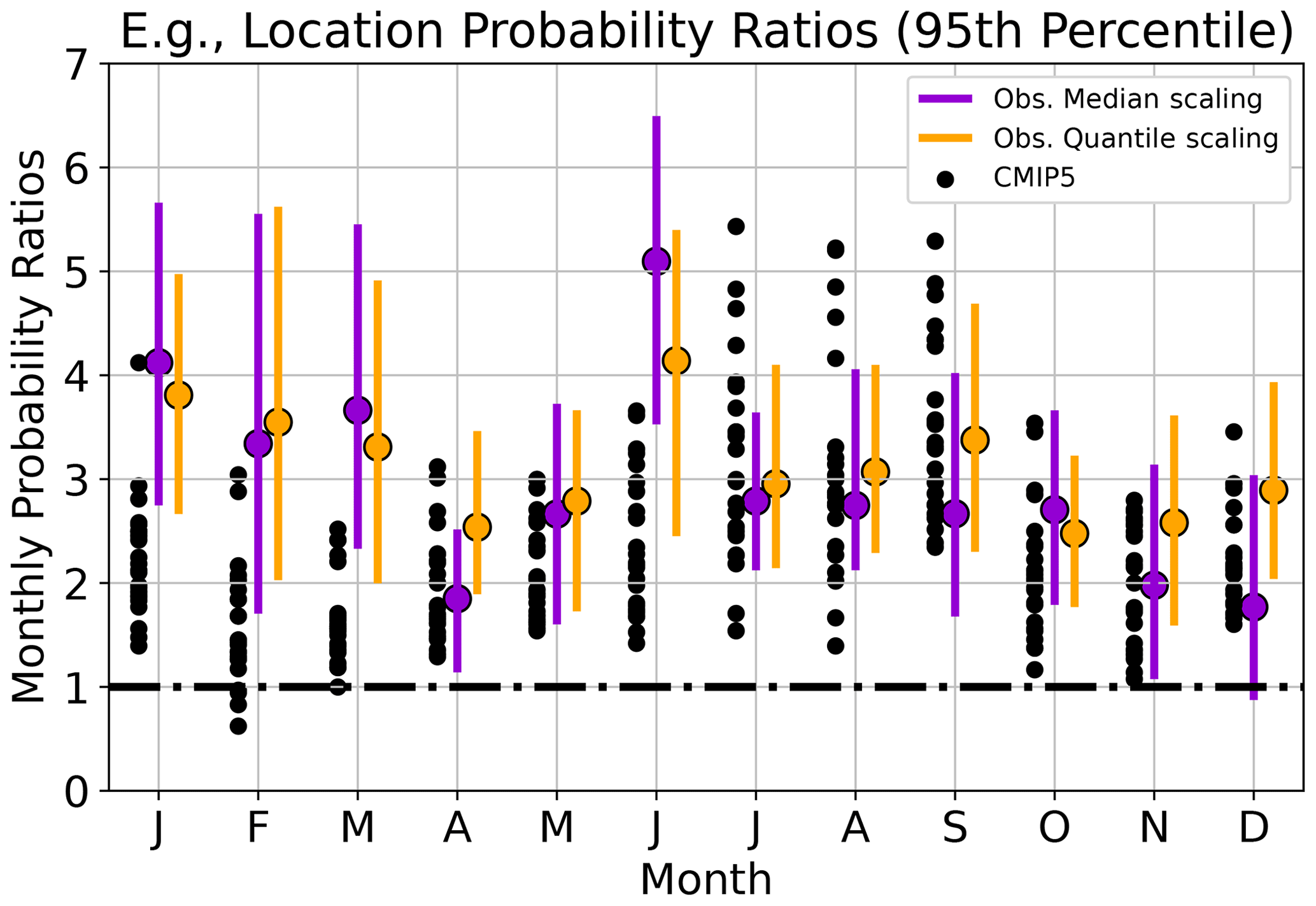
Figure 2 Seasonal cycles of probability ratios at the 95th percentile in Phoenix, calculated with the observation-based median-scaling (purple) and quantile-scaling (orange) methods and the model-based method (black). Purple and orange dots and bars show the median and 95 % confidence intervals for the observation methods, respectively; each black dot shows the PR of an individual model from the CMIP5 ensemble. The black dashed line at PR=1 is the boundary above which the probability of occurrence is greater in the human-forced climate than the counterfactual climate. Distributions with confidence intervals (or model ensemble estimates with all but one member) greater than PR=1 are statistically significant.

The model-based PR seasonal cycle exhibits a pattern consistent with other model attribution studies, showing an increasing seasonal temperature amplitude as the climate warms (Santer et al., 2018). Median- and quantile-scaling PRs show a less consistent seasonal pattern. Quantile-scaled monthly PRs are always ≥1.5 and have a limited seasonal amplitude (∼1.6 across the median estimates). The seasonal range of median-scaled PRs is twice as broad (∼3.2) and exhibits no coherent seasonal pattern. At times, the widths of PR confidence intervals calculated with the observation-based methods differ, with median-scaling confidence intervals often wider than those from quantile scaling. This distinction arises from a combination of physical and methodological factors. By design, the quantile-scaling method enables the variance in scaled distributions to shift with GMST. This variance shift – especially if the quantile-scale factors encourage broadening or narrowing in the tails – can become pronounced with large GMST mean changes (Appendix B; Eq. B2). Whereas the overland temperature variance (and hence of the upper-tail of temperature extremes) has ostensibly increased in recent decades (Seneviratne et al., 2016), the pattern of historical T_max variance change is spatially heterogeneous and often insignificant (Shen et al., 2011; Donat and Alexander, 2012; Lewis and King, 2017). Increases in the temperature variance are important for attribution assessment (they are the key feature captured by the quantile-scaling method), but they are not necessarily surprising. Temperature variance increases have theoretical grounding in atmospheric dynamics in the tropics (Byrne, 2021), and soil moisture feedbacks or vegetation changes in the extratropics (Schär et al., 2004; Diffenbaugh and Ashfaq, 2010; Seneviratne et al., 2013; Vogel et al., 2017; Vargas Zeppetello and Battisti, 2020). There is a clear trend of increasing T_max variance at the Phoenix-containing grid point, such that the scale factors of higher quantiles largely outpace those of lower quantiles. When this quantile pattern shifts the climatological distribution, it stretches the forced distribution and narrows the counterfactual distribution. The sharper counterfactual distribution results in a narrower distribution of absolute temperature thresholds across the quantile-scaled distributions associated with the 95th percentile (not shown), which limits the range of quantile-scaled PR values. In contrast, median-scaling preserves the shape of the underlying climatology, resulting in a broader range (i.e., more uncertain set) of possible PR values across most months, due to the range of uncertain scale factors. Note that, in July, Phoenix's quantile-scaling uncertainties are broader than those from median scaling, indicating that trends in the upper quantiles of Phoenix's July T_max distribution are noisier than in other months.

3.1.2 Application to July 2016

We now explore our framework's attribution assessment of daily T_max in Phoenix in July 2016 (Fig. 3). Maximum temperatures in this particular month were above average, but not extreme, ranging between 34.2 and 41.9 ^∘C (Fig. 3b–c; blue histogram/time series). All 31 d of July 2016 have T_max observations that fall below the absolute temperature threshold (42.7 ^∘C) defined from the climatological distribution at the monthly critical quantile (0.967). Median PR estimates calculated at this critical quantile from each method serve as a lower bound on the PR of July T_max values observed above 42.7 ^∘C. These lower bounds are 2.7, 5.1, and 3.3 from the median-scaling, quantile-scaling, and model-based methods, respectively.

Figure 3 Application of the attribution framework to July 2016 in Phoenix, Arizona, USA. (a) Counterfactual (left curves) and forced (right curves) empirical cumulative distributions functions of T_max; distributions are derived from the median-scaling (purple dashed curves), quantile-scaling (orange dashed curves), and CMIP5 model-based methods (black and gray curves). (b) July probability ratios calculated with each method, along with the observed July 2016 histogram of Phoenix T_max. (c) Daily probability ratios (unitless) calculated with each method and observed T_max (^∘C; blue curve) for each day in Phoenix during July 2016. Purple and orange dots and bars in panels (b) and (c) show the median and 95 % confidence intervals for the observation-methods, respectively. Each black dot shows the PR of an individual model from the CMIP5 ensemble. Light-black shading in panels (a) and (b) represents the region of maximum temperatures above which PRs are not assessed with our framework (see the text). The black dashed line at 1.0 is the boundary above which the probability of exceedance is greater in the human-forced climate than the counterfactual climate.

Empirical cumulative distribution functions (CDFs) from the observation-based (orange and purple curves) and model-based (black/gray curves) methods illustrate the attribution framework as it relates to Phoenix temperatures in July (Fig. 3a). Although there is a noticeable spread across each method's distribution – especially among CMIP5-forced CDFs – CDFs exhibit a clear shift in the probabilities between the counterfactual climate and the forced climate. Every method shows that the maximum temperatures increase across nearly the full range of quantiles in July. For instance, about 20 % of T_max values (i.e., a CDF value of 0.2) were 35 ^∘C or less in the counterfactual climate, which drops to ∼10 % in the forced distribution. The cumulative density of T_max at 35 ^∘C is about 0.55 in the counterfactual compared with 0.4 in the forced distribution. This translates to exceedance probabilities (i.e., 1−CDF) of 0.45 and 0.6 in the counterfactual and forced distributions, respectively. The result indicates that, in our current climate warmed by human-caused climate change, on average, observed July Phoenix maximum temperatures are attributively more likely to exceed 35 ^∘C 15 % more frequently than they would in the cooler counterfactual climate.

July 2016 probability ratios (Fig. 3b) are significant across the full range of observed T_max values (binned every 0.5 ^∘C), rendering the increase in likelihood of T_max for the whole month of July attributable to human-induced climate change. PR values increase monotonically with increasing temperature (except at the highest T_max values with the model-based method). A $T_{\max }\ge \mathrm{42}{}^{\circ }$C observation is on average $>\mathrm{3.1}\times$ more likely in the human-warmed climate than it would be in the counterfactual climate, whereas $T_{\max }\ge \mathrm{40}{}^{\circ }$C is about 2× more likely across the methods. Likewise, PR uncertainties for each method increase into the upper tail of the T_max distribution, arising from increased sensitivity to the tail shapes and densities of the individual forced and counterfactual distributions.

There is good agreement on the magnitude – and perfect agreement on the sign – of July Phoenix PR values from the framework's multiple methods. This leads to a consistent and statistically significant result of increasing frequency associated with every daily T_max observation in July 2016 (Fig. 3c). When T_max>40 ^∘C, the quantile-scaling method constantly produces higher median PR than the median-scaling method, which is broadly consistent with our finding that higher quantile temperatures increase more than lower quantile temperatures in Phoenix over the historical period – though the increased uncertainty from the quantile-based method casts doubt on the exact magnitude of the attribution estimate, particularly skewing towards the high end of PR values. Model-based PRs are strongly dependent on the individual model used to assess attribution, supporting the use of an ensemble of models in our attribution framework. In general, the model-based method has lower PRs in the far-right tail than the observation-based methods (T_max>42 ^∘C in Figs. 3c, 4, and S5–S7).

A final cohesive assessment of these framework results depends on the particular desired application. For example, the percentage of days with significantly attributable T_max is 100 % across all three methods, suggesting that the influence of human-driven climate change in July 2016 was robust and expansive in scope. Alternatively, the median July 2016 T_max was, across our methods, about 1.9× more likely to occur on average because of attributable human-driven climate warming. Or, on average across our methods, Phoenix's 90th percentile T_max in July under the forced climate is about 1.2 ^∘C warmer than it would be in the counterfactual climate. Regardless of the framing, our results shows a distinct robust signal of attribution across these above-average T_max values, highlighting the framework's capacity to identify and quantify daily attributable events, enabling timely climate communication.

3.2 Additional real-world examples: climate attribution on 27 July 2016

We further explore the framework results by examining the attribution estimates at multiple locations on a single day. Using Berkeley Earth gridded observations on 27 July 2016, we compare the Phoenix attribution calculations (Figs. 2–3) with estimates from the following six additional locations: Asunción (Paraguay), Bengaluru (India), Cape Town (South Africa), Mildura (Australia), Nairobi (Kenya), and Warsaw (Poland; Fig. S8). These locations span both hemispheres and each continent (except Antarctica), tropical and extratropical climates, and both developing and developed countries.

Table 1 Median and 95 % confidence intervals (CI) of probability ratios (PRs) associated with (a) the local July monthly mean daily exceedances of the 95th percentile (calculated from the monthly counterfactual distribution; see the text) or (b) the local observed T_max on 27 July 2016. Distributions with confidence intervals greater than PR=1 are statistically significant.

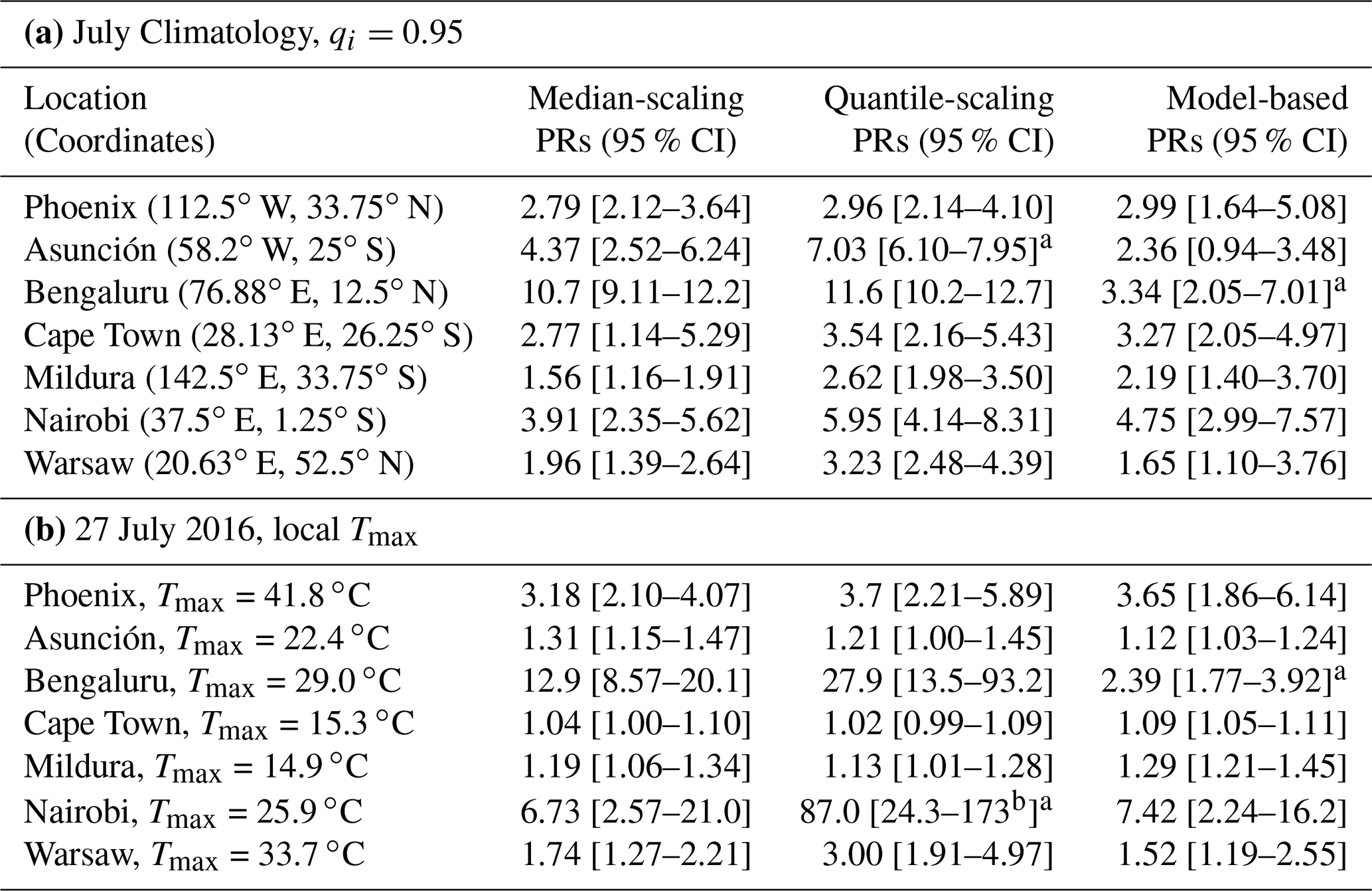
^a Indicates that the CI of a method's PR estimate differs significantly from the other two methods. ^b Indicates that the observed 27 July 2016 maximum temperature exceeded the local monthly critical quantile (0.967; see the text). In these cases, the reported PR is the value calculated at the critical quantile (Appendix C).

Table 1 shows each location's monthly (July) probability ratios (from each method) calculated at the 95th percentile (cf. July in Fig. 2) and PRs calculated with the observed nearest grid point maximum temperature on 27 July 2016 (see Fig. 3). July results show strong agreement on the sign of attributable change, where the probability of observing a daily T_max higher than the counterfactual distribution 95th percentile has significantly increased at each location. Large PR values in Bengaluru show the locally observed high sensitivity (PR≥9) of maximum temperature to anthropogenic global warming. At the other sites, observed maximum temperatures exceeding the counterfactual 95th percentile have increased by a factor of 1.5× to 8.0×.

In Asunción and Bengaluru, the three methods significantly disagree on the magnitude of attributable changes, with smaller model-based estimates than those from the observation-based methods. This lack of multi-method consensus (values marked with the superscript ^a in Table 1) indicates reduced confidence in the magnitude of attributable changes at these sites. A conservative operational application of these results might frame the lowest median estimate (i.e., model-based PRs in each case) as the basis for a final assessment, for further impact studies, or for communication with the public (see the discussion in Sect. 3.1.2).

PR values on 27 July 2016 show the wide variation of results that can arise from daily attribution calculations. Weather noise drives much of this local observed temperature variability, while the signal of anthropogenic warming acts to increase the baseline maximum temperatures and change the likelihoods of each daily temperature being observed. For instance, relatively high local temperatures in Bengaluru and Nairobi are associated with PR values ranging from 2.2 to 173, whereas relatively common local temperatures in Asunción, Cape Town, and Mildura are associated with attribution estimates that are either barely significant or insignificant, indicating little to no human influence on the likelihood of their maximum temperature on 27 July 2016. Warsaw and Phoenix attribution estimates are modest, indicating a clear and attributable human-driven increase in the probabilities of their warmer-than-average local temperatures on 27 July 2016 (Sect. 3.1.2).

Though not exhaustive, these examples illustrate the framework's capacity to provide a broad range of location-specific estimates of daily climate attribution, given a grid of observed or forecast maximum temperatures. When combined with environmental conditions from global forecasting models, future framework applications will use this capability to support concurrent and immediate worldwide operational estimates of attributable daily weather events.

3.3 Global attribution estimates

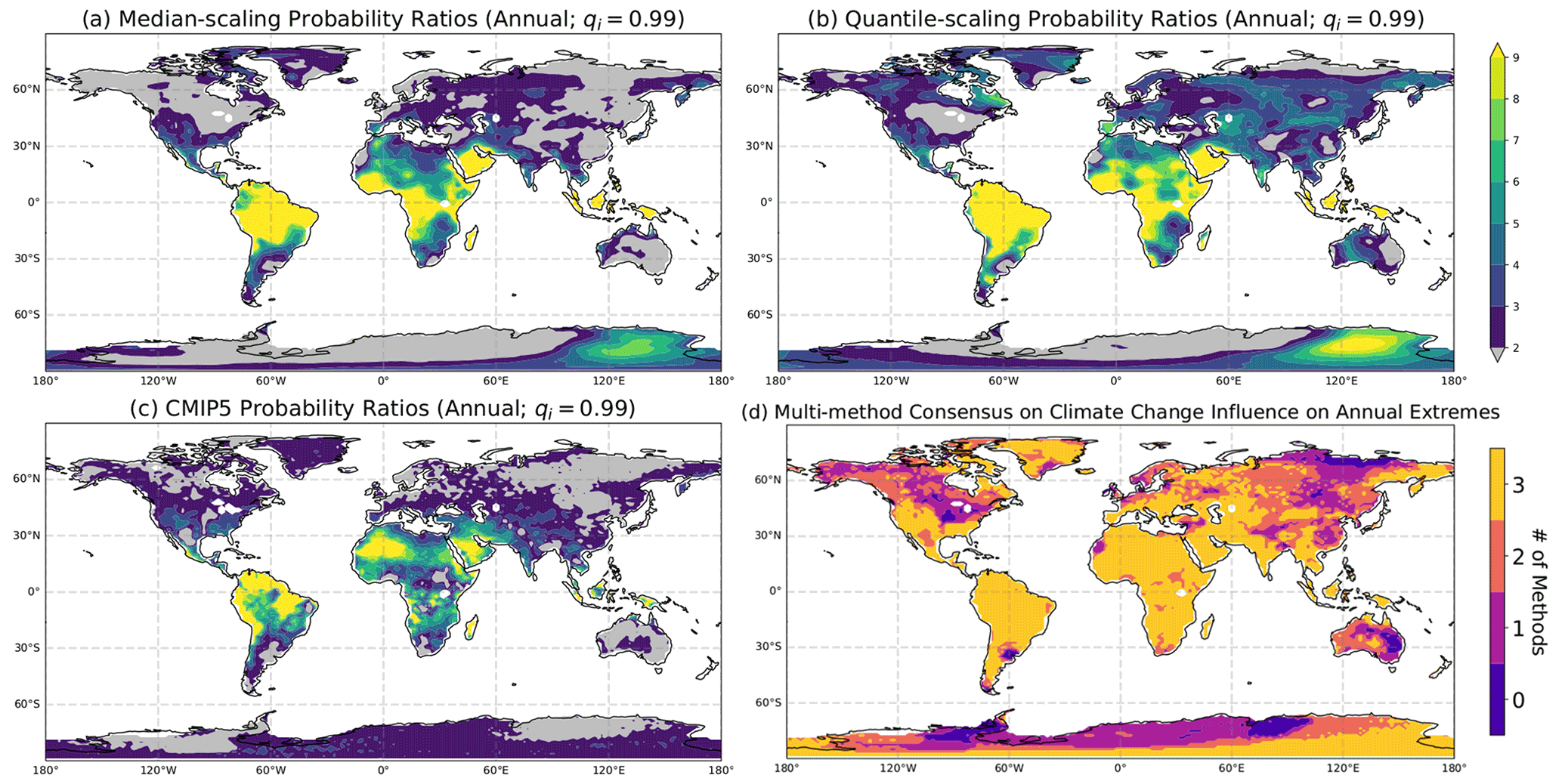
Figure 4 Globally resolved probability ratios (unitless) calculated with the observation-based (a) median-scaling approach, (b) quantile-scaling approach, and from (c) the ensemble mean of the model-based attribution approach. Analyses with PR<2 are grayed out to emphasize regions where human influence is most clearly found. (d) Map of the total number of the framework's attribution methods (derived from panels a–c) that have PR≥2 at each overland location (total between 0 and 3). PRs are found by comparing mean daily exceedances of the 99th percentile (calculated from the annual counterfactual distribution; see the text) between the full 31-year forced and counterfactual distributions from each method.

Moving on from these to location-specific examples to a complete global scale, we now demonstrate results from the attribution framework by mapping the probability ratios calculated at the annual 99th percentile of each counterfactual distribution. Probability ratios ≥2 occur across much of North America, Europe, central and southern Asia, Greenland, South America, parts of Australia, and even portions of Antarctica in each of the methods (Fig. 4a–c). By combining results from the framework's multiple methods, we are able to identify regions were we have strong confidence (indicated by consensus across methods) that extreme temperatures have become more likely due to human-caused climate change. We also determine which regions have attribution estimates that are sensitive to the methodologies or where the climate change signal is weaker. All three methods agree that the 99th percentile T_max has become at least twice as likely (compared with the counterfactual) over 56 % of the Earth's total land area (Fig. 4d). Over 80 % of the Earth's land area, at least two out of three methods agree that PR≥2 at these uncommon high-tail temperatures.

We find a coherent pattern of much higher probability ratios in the tropics that is consistent with time-of-emergence studies. In tropical regions, the anthropogenic signal of climate change dominates over small-amplitude weather noise, allowing human-influenced temperature trends to be detected earlier than in mid- and high latitudes (Mahlstein et al., 2011, 2012; Hawkins and Sutton, 2012; Frame et al., 2017). Observation-based PRs exceed 10 across the northern half of the South American continent, central Africa, the southern Arabian Peninsula, and Southeast Asia and Oceania. While multi-model mean PRs are smaller and less spatially coherent than observation-based estimates, they generally exhibit a similar pattern that appears to be shifted slightly northward (individual model results are presented for January and July in Figs. S9–S10). Taken together, our three methods agree that, across 52 % of tropical land (20^∘ S–20^∘ N), the probability of exceeding the 99th percentile of maximum temperatures has increased fivefold, while these probabilities have increased 10-fold over 9 % of tropical land. These findings illustrate our framework's ability to identify key global patterns of human-attributable influences in the climate system. It also underscores the framework's capacity to provide relevant global daily attribution estimates, with important implications for climate change communication, which we discuss below.

4 Summary and discussion

This study has detailed the development of a joint observational- and model-based (i.e., multi-method) framework to generate real-time estimates of the role that human-caused climate change plays in producing local daily temperatures around the globe. The framework is designed to be flexible across data sources and climatological state variables (especially those tied to climate warming through thermodynamics, e.g., temperature, sea level, and soil moisture; Trenberth et al., 2015), enabling its adaptation and expansion to a broad range of extremes and even relatively common weather characteristics. A key strength of our system is that it is computationally efficient, meaning that attributable changes in probability can be computed on the fly, using observations or forecasts. There are known regional and temporal gaps in the understanding and documentation of event attribution (Callaghan et al., 2021), yet lesser extreme daily events are nevertheless being altered by human-caused climate change. To this end, the framework developed here has focused primarily on these more common events which would be significantly rarer in a world without human-induced warming. In the future, this framework will support daily estimates of how human-caused climate change has influenced the likelihood of weather conditions at any location around the world, with immediate value for climate change communication.

Our methods are informed by state-of-the-art attribution guidelines from National Academies of Sciences report (National Academies of Sciences and Medicine, 2016) and the World Weather Attribution (van Oldenborgh et al., 2021) initiative. Specifically, the framework uses a hazard-based approach, framing attribution as the change in event probabilities responding to human-driven climate change (e.g., Jézéquel et al., 2018). Furthermore, the framework adopts objective selection criteria (based on exceedance thresholds defined by quantiles or absolute values of the state variable), relies on global mean surface temperature to define attributable human-influence on the climate system, uses a multi-method approach (including observations and bias-adjusted models) to generate multiple lines of evidence that may be combined for a consensus attribution analysis, employs resampling and model ensembles to assess estimate uncertainties, and is designed to be followed by clear and timely communication with the scientific community and the public.

Some procedural concessions have been made in this implementation. The framework is strictly statistical and is not able to consider the physical environment (e.g., synoptic conditions) during an event. It is currently unable to compute attribution estimates for dynamically driven extremes (such as extreme precipitation; Pfahl et al., 2017), although improved modeling and reconstruction of these events could eventually enable statistical historical attribution (Klein et al., 2021). Furthermore, this attribution framework is not intended to replace in-depth attribution studies for major extreme events. These events, including large-scale heat waves (e.g., Philip et al., 2021) and hurricane-driven heavy precipitation (Van Oldenborgh et al., 2017), not only involve complex event definitions (related to large-scale atmospheric conditions) but also often require extreme value statistics not implemented here (Coles, 2001). Our system also omits vulnerability and exposure analyses (e.g., Stone et al., 2021; van Oldenborgh et al., 2021). Instead, the framework is designed to be complementary and supportive to these studies. We see our system's potential to serve as an objective screening tool to identify events that warrant more complex analysis. Because our tool is focused on day-to-day weather conditions rather conditions that require extreme value theory, it serves as a lower bound on the attributable human influence on the observed conditions. After immediate assessment and identification with our framework, attribution estimates for an event could then be refined using more complex attribution approaches (e.g., Philip et al., 2021).

Several limitations warrant future investigation and improvement. The framework's observation-based attribution methods assume a historical linear-scaling relationship between the state variable and global mean surface temperature. Some research studies have shown that this relationship can be nonlinear, especially for high temperature extremes in the tropics (e.g., Chen et al., 2019). Our framework could be updated to model this complexity, allowing a more dynamic relationship between attributable global mean temperature changes and the associated state variable changes. Furthermore, because of the linear extrapolation involved in the observation-based scaling methods, historical and modern-day aerosols potentially mask attributable greenhouse-gas-driven warming (e.g., Van Oldenborgh et al., 2018; Seneviratne et al., 2021). Likewise, crop expansion, irrigation, and other land use practice have been shown to either amplify or (more often) mask regional heat extremes (e.g., Mueller et al., 2016a, b; Thiery et al., 2017; Findell et al., 2017; Thiery et al., 2020). Our current methods do not disentangle aerosol and land use masking from attributable greenhouse gas forcing. This could be addressed by screening observation-based estimates with model-based results (which can control for these forcings) – in cases where their patterns agree, nonlinearities from these processes are unlikely to be substantially affecting attribution assessments.

This study used a single state variable, the daily maximum temperature, to illustrate the attribution framework in action and a single set of observations and models – Berkeley Earth and CMIP5 – on a shared coarse grid. Because of this coarse grid, small-scale climate events in some regions may not be well represented. To limit biases arising from this scale discrepancy, extending this approach to a finer-scale grid or point-based observations may be required – particularly in operational contexts requiring location specificity. By design, the framework is agnostic of data sources and may be flexibly extended or adapted with different model ensembles (e.g., CMIP6; Eyring et al., 2016) and/or observational data sets. Point-based observations such as station data could be used to make highly localized estimates of how human-driven climate change is affecting the likelihood of certain events. In these cases, downscaling could be applied to gridded data during the bias-adjustment step (e.g., Lange, 2019) to enable harmonious interpretations across gridded and point-based estimates.

The multi-method approach herein could be applied to estimate attributable probability changes for other well-observed and well-modeled climatological state variables (e.g., precipitation), providing appropriate adaptations (e.g., variable-specific bias adjustment). Extending our framework to integrate other environmental state variables, particularly those that may exhibit weak or nonlinear relationships with global mean temperature changes, could require future work that differs from variable to variable.

Global climate attribution studies remain underdeveloped and underexplored. While projects like the World Weather Attribution initiative have provided prominent rapid assessments of the influence of human-induced climate change on daily weather characteristics, these studies are often ad hoc and geographically biased towards Europe or North America. A recent study (Callaghan et al., 2021) estimates that while 80 % of the global land area containing 85 % of the global population have partially attributable temperature and/or precipitation trends, there remain large regions of Earth (∼33 %; supporting 11 % of the global population) with relatively little study of attributable impacts; this is especially true in parts of Asia and western Africa. While a few studies have explored global attribution as is done herein (e.g., Huber and Knutti, 2012; Diffenbaugh et al., 2017; Sippel et al., 2020), there remain important gaps in both scientific investigation and public understanding of how climate change regularly affects local communities across the globe, which our method is designed to address.

Our sample global attribution analyses show a consistent pattern of strongly attributable human influences on maximum temperatures across the tropics. These results highlight important links between global inequities, climate data, and attribution of extreme temperatures. Although the tropical time series from Berkeley Earth are sufficiently long – 65+ years (Fig. S2) – for accurate estimates of attributable probability distributions changes (Sippel et al., 2021), historically poor quality data and limited ground-truthing of climate models makes the attribution more challenging in low-latitude regions (Otto et al., 2020). Additionally, these low-latitude regions of high climate signal-to-noise contain many developing populous countries that can be highly vulnerable to climate impacts (e.g., Frame et al., 2017; King and Harrington, 2018; Otto et al., 2020). Despite data limitations, consensus results among the methods from our framework show that more than half (52 %) of the tropical land area is 5 times more likely to high-tail probabilities of maximum temperature today because of human-caused climate change than it would have been in preindustrial times. Such explorations with our framework, coupled with impacts studies in the future, could provide ongoing and rapid insight into how human-driven climate change is inordinately influencing vulnerable tropical regions.

Public perceptions of climate risk are strongly tied to the effects of extreme weather (e.g., Berry et al., 2010; Sullivan and White, 2019, and references therein), but typically, the links between the observed weather and climate change are not quantified or are not available until weeks or months after an event occurs. Our new global attribution framework enables the careful study, documentation, and prompt communication of how climate change is altering the likelihood of both extreme and ordinary weather events. By providing an objective way of attributing changes to human influences on the climate system, our framework will put immediate attribution estimates into the hands of media and policymakers while an event is underway or even before it occurs. In those critical moments, our approach enables confident and timely discussions of climate change causes and impacts, in order to facilitate and strengthen public understanding.

Appendix A: Bias-adjustment methodology

Following Lange (2019), let $x_{\mathrm{cal}}^{\mathrm{sim}}$ be the model's simulated time series (sim) of the state variable of interest (x) over a defined calibration period (cal). Then $x_{\mathrm{cal}}^{\mathrm{obs}}$ is the observed time series (obs) of the state variable over the same calibration period, and likewise, $x_{\mathrm{adj}}^{\mathrm{sim}}$ is the simulated time series over the bias adjustment period (adj). The target distribution is a bias-adjusted distribution of the simulated state variable of interest over the adjustment period, ${\stackrel{\mathrm{̃}}{x}}_{\mathrm{adj}}^{\mathrm{sim}}$. The bias adjustment method is as follows:

1. Detrend $x_{\mathrm{cal}}^{\mathrm{obs}}$, $x_{\mathrm{cal}}^{\mathrm{sim}}$, and $x_{\mathrm{adj}}^{\mathrm{sim}}$. Linear trends are computed and removed on an annual timescale from each daily value of x.

2. Transfer the simulated climate change signal for every distribution quantile from $x_{\mathrm{cal}}^{\mathrm{sim}}$ and $x_{\mathrm{adj}}^{\mathrm{sim}}$ to $x_{\mathrm{cal}}^{\mathrm{obs}}$. Then define $x_{\mathrm{adj}}^{\mathrm{obs}}$ as the resulting time series of pseudo-observations over the adjustment period. Note that these are “pseudo-observations” because they extend into periods of record or climate pathways that have not been observed. This step follows an quantile-mapping process with additive trend preservation:

   1. Given a single daily observation, X from the time series $x_{\mathrm{cal}}^{\mathrm{obs}}$, we seek the corresponding pseudo-observation over the adjustment period, Y, to comprise part of $x_{\mathrm{adj}}^{\mathrm{obs}}$. Then we define $p=F_{\mathrm{cal}}^{\mathrm{obs}}\left(X\right)$ as the cumulative probability of X. Likewise, 𝒬 is the quantile function (i.e., the inverse CDF) of each distribution.

   2. For each X in $x_{\mathrm{cal}}^{\mathrm{obs}}$, we solve the following:

      $$\begin{array}{}\text{(A1)}& Y=X+{\mathcal{Q}}_{\mathrm{adj}}^{\mathrm{sim}}\left(p\right)-{\mathcal{Q}}_{\mathrm{cal}}^{\mathrm{sim}}\left(p\right),\end{array}$$

      such that a corresponding time series $x_{\mathrm{adj}}^{\mathrm{obs}}$ is comprised of each Y, which is translated from $x_{\mathrm{cal}}^{\mathrm{obs}}$ via the difference between the simulated distributions of the adjusted and calibration periods.

3. Use parametric quantile mapping to adjust the distribution of values in $x_{\mathrm{adj}}^{\mathrm{sim}}$, using the distribution of pseudo-observations in $x_{\mathrm{adj}}^{\mathrm{obs}}$. This is performed via the following quantile mapping equation:

   $$\begin{array}{}\text{(A2)}& {\stackrel{\mathrm{̃}}{X}}_{\mathrm{adj}}^{\mathrm{sim}}=\widehat{F}{{}_{\mathrm{adj}}^{\mathrm{obs}}}^{-\mathrm{1}}\left({\widehat{F}}_{\mathrm{adj}}^{\mathrm{sim}}\left(X_{\mathrm{adj}}^{\mathrm{sim}}\right)\right),\end{array}$$

   which bias adjusts each simulated daily value from the adjustment period time series ($X_{\mathrm{adj}}^{\mathrm{sim}}$) using a transform function consisting of parametrically fit observed and simulated distributions, ${\widehat{F}}_{\mathrm{adj}}^{\mathrm{obs}}$ and ${\widehat{F}}_{\mathrm{adj}}^{\mathrm{sim}}$, respectively. In this study, the parametric distributions of $x_{\mathrm{adj}}^{\mathrm{obs}}$ and $x_{\mathrm{adj}}^{\mathrm{sim}}$ are fit to T_max values, assuming that they are normal⁵. The resulting full time series of bias-adjusted data values (${\stackrel{\mathrm{̃}}{X}}_{\mathrm{adj}}^{\mathrm{sim}}$) over the adjustment period comprise ${\stackrel{\mathrm{̃}}{x}}_{\mathrm{adj}}^{\mathrm{sim}}$.

4. Restore the trend subtracted from $x_{\mathrm{adj}}^{\mathrm{sim}}$ to the bias-adjusted time series ${\stackrel{\mathrm{̃}}{x}}_{\mathrm{adj}}^{\mathrm{sim}}$.

In this study, bias adjustment is applied to each model's GMST time series and monthly T_max time series at each overland grid point. Berkeley Earth T_max observations over a calibration period of 1985–2015 are used to inform the T_max bias adjustment over the full time series at each overland location of each model and experiment. The adjustment periods are over 1975–2005 for natural experiment simulations and over 1880–2050 for forced experiment simulations, respectively. Note that, for each the 11 natural simulations, the trained quantile-mapping relationship between its paired historical plus projected time series (Table S1) and the observed time series is used to translate the natural simulations, i.e., $x_{\mathrm{adj}}^{\mathrm{sim}}$ is given by the natural distribution over 1975–2005, while $x_{\mathrm{cal}}^{\mathrm{sim}}$ and $x_{\mathrm{cal}}^{\mathrm{obs}}$ are still defined over the 1985–2015 calibration period. Illustrative comparisons between the raw and bias-adjusted simulated distributions in Phoenix (with an example model, GFDL CM3) are shown in Fig. S11. Global maps of bias adjustments demonstrating their range across individual models are provided at two quantiles in July in Fig. S12–S13. Note that this statistical bias-adjustment approach is univariate and inherently violates each model's physical consistency. Because of this drawback, the method should not be used as a precursor to conducting multivariate attribution analyses (e.g., heat stress indicators that rely on both temperature and humidity fields or coupled T_min/T_max analysis).

Appendix B: Scale factors

Following Philip et al. (2020), the scale factor, β, is equal to the slope of the linear least squares regression between the full time series of x (at a fixed longitude/latitude location; λ, ϕ) and annual GMST:

$$\begin{array}{}\text{(B1)}& \mathit{\beta }=r\times {\displaystyle \frac{s_x}{s_{\mathrm{GMST}}}},\end{array}$$

where r is the correlation coefficient between x and GMST, and s are their respective standard deviations.

An observed climatological distribution of the state variable over an arbitrary time period (taken herein to be 1985–2015) is given by x(t_i→ii), and the temporal mean GMST over that same time period is $\stackrel{\mathrm{‾}}{\mathrm{GMST}\left(t_{i\to ii}\right)}$. To translate this distribution to a different time period, the distribution is shifted by the scaled GMST mean difference between the climatology, and the new period is as follows:

$$\begin{array}{}\text{(B2)}& x\left(t_{j\to jj}\right)=x\left(t_{i\to ii}\right)+\mathit{\beta }\times \mathrm{\Delta }\mathrm{GMST},\end{array}$$

where x(t_j→jj) is the scaled distribution of the state variable and where

$$\mathrm{\Delta }\mathrm{GMST}=\stackrel{\mathrm{‾}}{\mathrm{GMST}\left(t_{j\to jj}\right)}-\stackrel{\mathrm{‾}}{\mathrm{GMST}\left(t_{i\to ii}\right)}.$$

Note that the scaling approach retains the full range of interannual variability present in the underlying climatology.

Appendix C: Discrete probability ratio calculations

At a given quantile in the counterfactual distribution, q_i, the discrete calculation of the probability ratio is as follows:

$$\begin{array}{}\text{(C1)}& {\mathrm{PR}}_t\equiv {\displaystyle \frac{p_{\mathrm{forced}}}{p_{\mathrm{cf}}}}={\displaystyle \frac{\sum _{d=\mathrm{1}}^{N_t}H\left(T_{\max }\right(d)-T_{q_i})}{N_{E,t}}},\end{array}$$

where H(⋅) is the Heaviside step function, T_max(d) is a daily maximum temperature sampled from a forced distribution, $T_{q_i}$ is an absolute temperature threshold defined by the quantile from the counterfactual distribution, d is the day index, and N_t is the number of days over the timescale we are considering. The expected value of the (E[⋅]) number of days that will exceed the temperature threshold over a given timescale comes directly from the definition of the percentile, as follows:

$$\begin{array}{}\text{(C2)}& N_{E,t}\equiv E\left[\sum _{d=\mathrm{1}}^{N_t}H\left(T_{\max }\left(d\right)-T_{q_i}\right)\right]=N_t\times \left(\mathrm{1}-q_i\right).\end{array}$$

For example, the expected number of days exceeding the 95th percentile (q_i=0.95) on a yearly timescale (N_year=365 d) is $N_{E,\mathrm{year}}=\mathrm{18.25}$ d (Table S2). Likewise, the threshold subceedance is given by $N_t-N_{E,t}$. This estimate is used to define the critical quantile for appropriate assessment with our discrete counts methodology; it is given by $N_{E,t}=\mathrm{1}$ (Sect. 2.4). Note that, when PR_t>1, then p_forced is increased relative to p_cf by a factor of PR_t. The absolute temperature threshold at a specific quantile, $T_{q_i}$, may also be calculated from the climatology rather than the counterfactual distribution. In this case, p_cf becomes $\sum _{d=\mathrm{1}}^{N_t}H\left(T_{\max ,\mathrm{cf}}\right(d)-T_{q_i})$, where T_max,cf is the counterfactual distribution of daily maximum temperatures.

Our final estimate of the attributable probability ratio is given by the mean over every year's individual probability ratio values, i.e., $\stackrel{\mathrm{‾}}{{\mathit{\eta }}_t}=E\left[{\mathit{\eta }}_{t_{\mathrm{1}\to \mathrm{31}}}\right]$. The mean change in the number of days between the forced distribution and counterfactual is $\stackrel{\mathrm{‾}}{{\mathit{\delta }}_t}=\stackrel{\mathrm{‾}}{{\mathit{\eta }}_t}\times N_{E,t}-N_{E,t}$.