Evaluation of simulated responses to climate forcings: a flexible statistical framework using confirmatory factor analysis and structural equation modelling – Part 2: Numerical experiment

The performance of a new statistical framework, developed for the evaluation of simulated temperature responses to climate forcings against temperature reconstructions derived from climate proxy data for the last millennium, is evaluated in a so-called pseudo-proxy experiment, where the true unobservable temperature is replaced with output data from a selected simulation with a climate model. Being an extension of the statistical model used in many detection and attribution (D&A) studies, the framework under study involves two main types of statistical models, each of which is based on the concept of latent (unobservable) variables: confirmatory factor analysis (CFA) models and structural equation modelling (SEM) models. Within the present pseudo-proxy experiment, each statistical model was fitted to seven continental-scale regional data sets. In addition, their performance for each defined region was compared to the performance of the corresponding statistical model used in D&A studies. The results of this experiment indicated that the SEM specification is the most appropriate one for describing the underlying latent structure of the simulated temperature data in question. The conclusions of the experiment have been confirmed in a cross-validation study, presuming the availability of several simulation data sets within each studied region. Since the experiment is performed only for zero noise level in the pseudo-proxy data, all statistical models, chosen as final regional models, await further investigation to thoroughly test their performance for realistic levels of added noise, similar to what is found in real proxy data for past temperature variations.

1 Introduction

The evaluation of climate models used to make projections of future climate changes is a crucial issue within climate research (Flato et al., 2013). Depending on the scientific question and the characteristics of the climate model under study, evaluation approaches may employ various statistical methods possessing different degrees of complexity. For example, model performance can be assessed visually comparing maps or data plots describing both the climate model outputs and the observations (see, for example, Braconnot et al., 2012) or calculating various metrics summarising how close the simulated values of the climate variable of interest are to the corresponding observed ones, for example, (i) a simple root mean square as given in Goosse et al. (2015), Sect. 3.5, (ii) the kappa statistic in Texier et al. (1997), and (iii) the Hagaman distance used by Brewer et al. (2007a, b).

Other studies may instead focus on comparing the probability distributions of climate model output to the corresponding empirical distributions of observed data using so-called divergence functions (Thorarinsdottir et al., 2013). It is also possible to validate climate models by modelling joint distributions for more than one climatic variable, as was done by Philbin and Jun (2015), where the near-surface temperature and precipitation output from decadal runs of eight atmospheric ocean general circulation models (AOGCMs) has been validated against observational proxy data. The term “proxy data” refers to substitute data for direct instrumental measurements of physical climate variables, such as temperature or precipitation, that have been obtained from various natural climate “archives” such as tree rings, corals, ice cores, and cave speleothems and which can be statistically calibrated to represent the desired climate variables (e.g. Jones et al., 2009).

It should be emphasised that evaluation of climate model simulations is a complex process requiring the performance of a large number of tests with respect to various climatological aspects. As pointed out by, for example, Flato et al. (2013) and Goosse et al. (2015), no individual evaluation technique is considered superior, leading to a final, definitive product. The model should be continuously retested as new data or experimental results become available. A model is sometimes said to be validated if it has passed a reasonable number of tests. In such a case, the credibility of model projections performed with such a climate model could be very high.

Recently, a new framework for evaluation of climate model simulations against observational data was developed by Lashgari et al. (2022) (henceforth referred to as LAS22). The framework contains statistical models with latent variables, namely confirmatory factor analysis (CFA) models and structural equation modelling (SEM) models. Focusing on a near-surface temperature as a climatic variable of interest, all statistical models within LAS22 are developed for use with data from a single region of any size. Data are supposed to cover (approximately) the last millennium, which implies that observational data contain not only instrumental observations, but also reconstructions derived from climate proxy data.

Another climate-relevant property of the LAS22 framework is that it distinguishes between external climate factors that can be either of natural or anthropogenic origin and the internal climate processes that are internal to the climate system itself (Kutzbach, 1976). Examples of external natural factors are changes in solar radiation, changes in the orbital parameters of the Earth, and volcanic eruptions. External climate factors of anthropogenic origin include, for example, the ongoing release of carbon dioxide to the atmosphere, primarily by burning fossil fuels, the emissions of aerosols through various industrial and burning processes, and changes in land use (Jungclaus et al., 2017). Among the internal climate processes, we can name ocean and atmosphere circulation and their variations and mutual interactions.

LAS22 also uses the concept of radiative forcing, defined as the net change in the Earth's radiative balance at the tropopause (incoming energy flux minus outgoing energy flux expressed in watts per square metre (W m⁻²). Sometimes scientists use the term climate forcing instead of radiative forcing (Liepert, 2010). In what follows, we simply write just forcing.

Concerning its statistical properties, the LAS22 framework can be viewed as a natural extension of the statistical model used in so-called detection and attribution (D&A) studies (see, for example, Bindoff et al., 2013). This statistical model, often associated with “optimal fingerprinting” techniques (see, for example, Allen and Stott, 2003), is known among statisticians as a measurement error (ME) model (or, equivalently, an errors-in-variables model). Its application within D&A studies allows researchers to address the two main questions, namely the question of detection of observed climate change and the question of its attribution to real-world forcings. Importantly, the question of attribution cannot be addressed without simultaneously addressing the question of consistency between simulated and observed climate change.

Using the fact that a general ME model is a special case of CFA and SEM models, LAS22 has extended the ME model specification to more complicated CFA and SEM models. As a result, it became possible to overcome some limitations of the ME model, for example, the inability to take into account the effects of possible interactions between forcings (see, for example, Marvel et al., 2015; Schurer et al., 2014), or the inability to account for non-climatic noise in the observational data, or the estimation instability arising under the so-called “weak-signal” regime (DelSole et al., 2019).

In addition, LAS22 allows for a flexible specification of latent structure of observable variables, depending on aspects such as (i) the number of forcings used to drive the climate model under consideration, (ii) our knowledge and/or assumptions about their possible effects on the temperature within the region and period of interest, (iii) assumptions concerning co-relations among model variables representing both latent and observable temperatures, and (iv) the availability of simulated data.

At the same time, the LAS22 framework also makes it possible to address the questions posed in D&A studies. Moreover, LAS22 allows the attribution issue to be addressed separately from the question of consistency.

The latter feature is due to another framework, whose ideas were used by LAS22 during the course of extension of the ME model specification. Developed by Sundberg et al. (2012), the design of the second framework (henceforth referred to as SUN12) allows for the comparison of climate model simulations and proxy data for the relatively recent past of about 1 millennium. As the main result, SUN12 formulated two test statistics: a correlation and a distance-based test statistic (for their applications see Hind et al., 2012; Hind and Moberg, 2013; Moberg et al., 2015; PAGES2k-PMIP3 group, 2015; Fetisova, 2015).

In the present work, we, part of the LAS22 research team, aim to perform a practical evaluation of the statistical models of LAS22 in a numerical experiment. In addition, we also aim to compare their performance to the performance of the ME model used in D&A studies when it is applied to the same data.

A vital feature of our numerical experiment is that specially selected climate model simulations replace real-world temperature observations. Experiments using climate model simulations instead of real-world data are often referred to in the (paleo)climatological literature as pseudo-proxy experiments (PPEs). An example of PPEs is the kind of experiments that aim to evaluate the performance of statistical methods used to reconstruct past climate variations from climate proxy data (for its description see Smerdon, 2012).

Importantly, climate model simulations that played the role of observational data were forced by the same reconstructed forcings as those that are subject to evaluation. This condition justifies the consistency (both in terms of the magnitude and large-scale shape) between the unobservable simulated temperature responses to the forcings of interest, embedded in the simulations, and their counterparts, embedded in pseudo-observations.

Thus, the rejection of the statistical model in question should be interpreted as an unambiguous indication of the associated underlying latent structure being misspecified and inconsistent with the data. Contrarily, a statistical model that is not rejected and demonstrates the best fit among all models with an admissible and climatologically defensible solution can be chosen as a final model, providing an adequate description of the underlying latent structure.

It is important to add that our pseudo-observations play the role of the true unobservable temperature, uncontaminated by any non-climatic noise. Although it is of great interest to evaluate the sensitivity of the statistical models under consideration to increasing noise levels, no such sensitivity analysis was performed within the confines of the present experiment.

After having investigated which statistical models that demonstrate an acceptable performance with zero proxy noise, it will be easier to design the future sensitivity analysis.

Concerning statistical packages, in the present work we employed the R package sem (see Fox et al., 2014, http://CRAN.R-project.org/package=sem, last access: 11 November 2022) using R version 3.0.2 (R Core Team, 2013) for estimation of all statistical models under study. For derivation of symbolic expressions of the reproduced variance–covariance matrices associated with our statistical models under different hypotheses, we used MATLAB (R2017a).

Finally, let us describe the structure of this paper. Section 2 provides a description of the data, the results of its initial analysis, and the way of constructing data sets to which we fit our statistical models. The statistical models from the LAS22 framework are presented in Sect. 3, while the numerical results of their analyses are given partly in Sect. 4 and partly in the first section of the Supplement to this article. In total, the Supplement contains three sections. Its second section is devoted to providing a theoretical overview of the central definitions and concepts of SEM, which includes CFA as its special case. In the third section of the Supplement, one finds examples of using the R package sem and MATLAB. The main findings of our numerical study are presented and discussed in this article, Sect. 5.

2 Description of simulated data and its initial analysis

Data analysed in the present study consist of simulated near-surface temperatures generated with the Community Earth System Model (CESM) version 1.1 for the period 850–2005 (the CESM-LME (Last Millennium Ensemble)). A detailed description of the model and the ensemble simulation experiment can be found in Otto-Bliesner et al. (2016) and references therein.

For our analysis, we select seasonal-mean temperature data for the seven regions and the seasons defined by the PAGES 2k Consortium (2013), labelled Europe, the Arctic, North America, Asia, South America, Australasia, and Antarctica. As seen in Fig. 1 in their paper, the continental regions are not exactly the same as the continents themselves. Moreover, both land and sea surface temperatures are included in three of the regions (Arctic, North America, Australasia), while land-only temperatures are used in the other four. Note also that the choice of seasons differs among the regions, depending on what was considered by the PAGES 2k Consortium (2013) as being the optimal calibration target for the climate proxy data they used. Annual-mean temperatures were used for the Arctic, North America, and Antarctica, while some warm-season temperatures are used for Europe (JJA), Asia (JJA), South America (DJF), and Australasia (September–February). The set of simulation temperature data sequences that we use here is a subset of the dataset published by Moberg and Hind (2019).

The CESM-LME experiment used 2^∘ resolution in the atmosphere and land components and 1^∘ resolution in the ocean and sea ice components. To extract seasonal temperature data from this simulation experiment such that they correspond to the seven regions defined in the PAGES 2k Consortium (2013) study, we followed exactly the same procedure as in the model vs. data comparison study undertaken by the PAGES2k-PMIP3 group (2015). After extraction, our raw temperature data sequences have a resolution of one temperature value per year. The time period analysed here is the 1000-year-long period 850–1849 CE. The industrial period after 1850 CE has been omitted in order to avoid a complication due to the fact that the CESM simulations for this last period include ozone-aerosol forcing, which is not available for the time before 1850. Below, we list all simulated temperature sequences available within each region and the period of interest. We also describe the key characteristics of the associated reconstructed forcings (a detailed description and time-series plots of forcing data can be found in Fetisova et al., 2017):

1. {x_Sol t} is forced only with a reconstruction of the transient evolution of total solar irradiance. This is a measure of the averaged amount of radiated energy from the Sun that reaches the top of the atmosphere of the planet Earth during a year. See Fig. S4.1 in Fetisova et al. (2017). Within each region, there are four sequences forming the x_Sol ensemble.

2. {x_Orb t} is forced only with changes in the boundary conditions due to the transient evolution of the Earth's orbital parameters, i.e. the seasonal and latitudinal distribution of the orbital modulation of insolation. According to Fig. S4.3 in Fetisova et al. (2017), the temporal evolution of the orbital forcing varies with region and season. Within each region, there are three replicates of x_Orb forming the x_Orb ensemble.

3. {x_Volc t} is forced only with a reconstruction of the transient evolution of volcanic aerosol loadings in the stratosphere, as a function of latitude, altitude, and month. According to Fig. S4.4 in Fetisova et al. (2017), the temporal evolution of the volcanic forcing varies with region. Within each region, there are five replicates of x_Volc forming the x_Volc ensemble.

4. {x_{Land (anthr) t}} is forced only with a reconstruction of the transient evolution of anthropogenic land use, i.e. changes particularly in fractional areas of crops and pasture within each grid cell on land. The type of natural vegetation has been prescribed in each grid cell and held constant at pre-industrial levels. According to Fig. S4.5 in Fetisova et al. (2017), the reconstruction of the (anthropogenic) land forcing varies with region. Within each region, there are three replicates of x_{Land (anthr)} forming the x_{Land (anthr)} ensemble. The CESM-LME climate model did actually include a dynamic land model (CLM4), which impacts the simulated climate through seasonal and interannual changes in the vegetation phenology¹ (Lawrence et al., 2012). Here, we interpret this as a possible contribution to internal random variability but not as a climate forcing. In the context of our framework, this assumption motivates the modelling of the simulated temperature response to the land forcing as a one-component temperature response containing only the simulated temperature response to reconstructed anthropogenic changes in land use.

5. {x_GHG t} is forced only with a reconstruction of the transient evolution of well-mixed greenhouse gases, GHGs, namely CO₂, N₂O, and CH₄. Prescribed reconstructed greenhouse gas concentrations, adopted from Schmidt et al. (2011), are derived from high-resolution Antarctic ice cores (see Fig. S4.2 in Fetisova et al., 2017). This makes it reasonable to assume that this reconstruction can contain information about both natural and anthropogenic influences. Hence, in contrast to the simulated temperature response to the land forcing, the simulated temperature response to the GHG forcing is modelled in our statistical framework as a two-component temperature response containing the simulated temperature response to anthropogenic changes and the simulated temperature response to natural changes in the GHG forcing. Within each region, there are three replicates of x_GHG forming the x_GHG ensemble.

6. {x_comb t} is forced by all above-mentioned single forcings together. Within each region, the x_comb ensemble consists of 10 replicates.

Regarding the GHG forcing in the climate model simulations studied here, some important aspects should be highlighted:

• The GHG forcing was implemented so that variations in greenhouse gas concentrations in the climate model's atmosphere are the same everywhere. This, however, does not imply that the simulated temperature response to the forcing is expected to be the same for all above-described regions and seasons.

• The climate model did not include an interactive carbon cycle model. This means that variations in the amount of greenhouse gases in the model’s atmosphere could not arise dynamically in response to changes in the model’s climate but only to variations determined by the reconstructed GHG forcing data. Consequently, if a SEM model suggests the existence of any causal path to the variable denoting the simulated temperature response to the GHG forcing, then such a path may be interpreted as an indication that interaction between climate and greenhouse gas concentrations has happened in the real climate system and that this interaction is reflected in the reconstructed GHG forcing history used to drive the climate model.

• Natural variations in greenhouse gas concentrations in the atmosphere occur on all timescales and are expected

  to have occurred during our entire study period. It is evident that anthropogenic activity has led to increased greenhouse gas concentrations in about the last 100 years of our study period, mainly due to combustion of fossil fuels. However, an anthropogenic influence on greenhouse gas concentrations may have started already several thousand years ago, although this possible influence has been debated. It can anyway not be excluded that human activity may have led to changes in GHG forcing throughout our entire study period (see discussion in Ciais et al., 2013, and references therein).

Prior to analysing the climate model simulations above by means of our statistical models, it is necessary to check whether each of the sequences satisfies the assumptions of these statistical models. To this end, an initial data analysis is performed, whose results are described in the next subsection.

2.1 Initial data analysis: checking assumptions

Let {x_{𝚏 repl.i t}}, where f ∈{ Sol, Orb, Volc, Land (anthr), GHG, comb }, $i=\mathrm{1},\mathrm{2},\mathrm{\dots },k_{\mathtt{\text{f}}}$, and t=850 CE, 851 CE, …, 1849 CE, represent the ith member (or, in the statistical parlance, replicate) within the x_𝚏 ensemble.

According to LAS22, the mean-centred x_{𝚏 repl.i t} is decomposed into forced and unforced components as follows:

$$\begin{array}{}\text{(1)}& x_{\mathtt{\text{f}}\mathrm{repl}.it}={\mathit{\xi }}_{\mathtt{\text{f}}t}^{\mathrm{S}}+{\stackrel{\mathrm{̃}}{\mathit{\delta }}}_{\mathtt{\text{f}}\mathrm{repl}.it},\end{array}$$

where ${\mathit{\xi }}_{\mathrm{f}t}^{\mathrm{S}}$ is the simulated temperature response to the reconstructed forcing f, i.e. the forced component, and ${\stackrel{\mathrm{̃}}{\mathit{\delta }}}_{\mathtt{\text{f}}\mathrm{repl}.it}$ is the simulated internal random temperature variability, including any random variability due to the presence of the forcing f, i.e. the unforced component. The forced and unforced components are assumed to be mutually independent.

In contrast to the random ${\stackrel{\mathrm{̃}}{\mathit{\delta }}}_{\mathtt{\text{f}}\mathrm{repl}.it}$, the temperature response ${\mathit{\xi }}_{\mathtt{\text{f}}t}^{\mathrm{S}}$ is treated as repeatable, or more precisely, as repeatable outcomes of random variables, assumed to be normally and independently distributed with zero mean and variance ${\mathit{\sigma }}_{{\mathit{\xi }}_{\mathtt{\text{f}}}^{\mathrm{S}}}^{\mathrm{2}}$. The repeatedness is motivated by the fact that all replicates within one and the same ensemble were forced by the same reconstructed forcing f, which generates the same ${\mathit{\xi }}_{\mathtt{\text{f}}t}^{\mathrm{S}}$ across all replicates within each ensemble.

Thus, the assumptions to check are the assumptions of normality and of mutually independent observations. Since the forced component of simulated temperatures is treated as a repeatable outcome, both assumptions concern the ${\stackrel{\mathrm{̃}}{\mathit{\delta }}}_{\mathtt{\text{f}}\mathrm{repl}.i}$ sequences. Since none of them is directly observable, the series to analyse are

$$\begin{array}{}\text{(2)}& \mathit{\{}{x}_{\mathtt{\text{f}}\mathrm{repl}.it}-{\stackrel{\mathrm{‾}}{x}}_{\mathrm{f}\text{.}t}\mathit{\}},\end{array}$$

where ${\stackrel{\mathrm{‾}}{x}}_{\mathrm{f}\text{.}t}$ denotes the average of k_𝚏 replicates at a time point t.

The independence assumption is checked by studying the autocorrelation structure of sequences, defined in Eq. (2), for each f and i. To reduce autocorrelation, which is typical for temperature data with annual resolution, a temporal aggregation of each time series was performed by taking m-year nonoverlapping averages for several values on m. Figures S1.1–S1.42 in Fetisova et al. (2017) show the resulting sample autocorrelation functions for four time average units, m=1, 5, 10, and 20 years.

According to these figures, m=5 could be motivated within some regions, for example, Asia and North America because at least 91 % of the autocorrelation coefficients are insignificant as they are within the 90 % confidence bounds. Nevertheless, it was decided to choose m=10 for all seven regions because the temperature responses to the forcings are more likely to exhibit a stronger autocorrelation for m=5 than for m=10. This can have a negative impact on the statistical properties of the parameter estimates of the statistical models analysed here. The time unit of 20 years was not applied because it reduces the sample size to 50 observations, which is too small for estimating the statistical models of interest (for discussions about appropriate sample sizes see Westland, 2015, and references therein).

To conclude, all x_{𝚏 repl.i} sequences analysed further are decadally resolved, implying that each of them contains 100 observations of 10-year mean temperatures. Time-series graphs that illustrate the resulting x_{𝚏 repl.i} sequences are shown in Figs. S2.1–S2.7 in Fetisova et al. (2017).

Further, we investigated whether the decadally resolved residual sequences, defined in Eq. (2), follow a normal distribution. Examination of the estimated density functions graphically (see Figs. S3.1–S3.7 in  Fetisova et al., 2017) did not reveal any obvious departures from the normal distribution. This conclusion was also supported by the Shapiro–Wilk test (Shapiro and Wilk, 1965), whose results, however, are not shown.

An important premise of the statistical models, suggested by LAS22, is that the variance of each ${\stackrel{\mathrm{̃}}{\mathit{\delta }}}_{\mathtt{\text{f}}\text{repl.}i}$ is known a priori. To this end, LAS22 employs the following independent estimator, applied to time-aggregated time series:

$$\begin{array}{}\text{(3)}& {\mathit{\sigma }}_{{\stackrel{\mathrm{̃}}{\mathit{\delta }}}_{\mathtt{\text{f}}}}^{\mathrm{2}}={\displaystyle \frac{{\sum }_{t=\mathrm{1}}^n{\sum }_{i=\mathrm{1}}^{k_{\mathtt{\text{f}}}}(x_{\mathtt{\text{f}}\mathrm{repl}.it}-{\stackrel{\mathrm{‾}}{x}}_{\mathrm{f}\text{.}t}{)}^{\mathrm{2}}}{n(k_{\mathtt{\text{f}}}-\mathrm{1})}},k_{\mathtt{\text{f}}}\ge \mathrm{2},\end{array}$$

requiring that (i) the variances of the ${\stackrel{\mathrm{̃}}{\mathit{\delta }}}_{\mathtt{\text{f}}\mathrm{repl}.i}$ are equal across all replicates within an ensemble, i.e. ${\mathit{\sigma }}_{{\stackrel{\mathrm{̃}}{\mathit{\delta }}}_{\mathtt{\text{f}}\text{repl.}i}}^{\mathrm{2}}={\mathit{\sigma }}_{{\stackrel{\mathrm{̃}}{\mathit{\delta }}}_{\mathtt{\text{f}}}}^{\mathrm{2}}$; (ii) the ${\stackrel{\mathrm{̃}}{\mathit{\delta }}}_{\mathtt{\text{f}}\mathrm{repl}.it}$ sequences within an ensemble are mutually uncorrelated across all k_𝚏 replicates; and (iii) the amplitude of the forcing effect is the same for each ensemble member.

If these assumptions are met, it will be possible not only to apply estimator (3), but also to build mean sequences by averaging over ensemble members. The usage of mean sequences is especially appreciated when the effect of a given forcing is expected to be weak.

If, on the other hand, these assumptions are violated, estimator (3) may result in a biased estimate, and the building of mean sequences becomes unmotivated. As a possible way to check whether these assumptions are violated or not and, in addition, to obtain an alternative estimate of ${\mathit{\sigma }}_{{\stackrel{\mathrm{̃}}{\mathit{\delta }}}_{\text{f}}}^{\mathrm{2}}$, LAS22 proposes to fit the following k_𝚏 indicator one-factor model, abbr. CFA(k_𝚏,1) model, to each ensemble:

$$\begin{array}{}\text{(4)}& \begin{array}{rcrcl}{x}_{\mathtt{\text{f}}\mathrm{repl}.1t}& =& {\mathit{\alpha }}_{\mathtt{\text{f}}}\cdot {\stackrel{\mathrm{̃}}{\mathit{\xi }}}_{\mathtt{\text{f}}t}^{\mathrm{S}}& +& {\stackrel{\mathrm{̃}}{\mathit{\delta }}}_{\mathtt{\text{f}}\mathrm{repl}.1t}\\ x_{\mathtt{\text{f}}\mathrm{repl}.2t}& =& {\mathit{\alpha }}_{\mathtt{\text{f}}}\cdot {\stackrel{\mathrm{̃}}{\mathit{\xi }}}_{\mathtt{\text{f}}t}^{\mathrm{S}}& +& {\stackrel{\mathrm{̃}}{\mathit{\delta }}}_{\mathtt{\text{f}}\mathrm{repl}.2t}\\ \mathrm{⋮}& & \mathrm{⋮}& & \mathrm{⋮}\\ x_{\mathtt{\text{f}}\mathrm{repl}.k_{\mathtt{\text{f}}}t}& =& {\mathit{\alpha }}_{\mathtt{\text{f}}}\cdot {\stackrel{\mathrm{̃}}{\mathit{\xi }}}_{\mathtt{\text{f}}t}^{\mathrm{S}}& +& {\stackrel{\mathrm{̃}}{\mathit{\delta }}}_{\mathtt{\text{f}}\mathrm{repl}.k_{\mathtt{\text{f}}}t},\end{array}\end{array}$$

where ${\stackrel{\mathrm{̃}}{\mathit{\xi }}}_{\mathtt{\text{f}}t}^{\mathrm{S}}={\mathit{\xi }}_{\mathtt{\text{f}}t}^{\mathrm{S}}/\sqrt{{\mathit{\sigma }}_{{\mathit{\xi }}_{\mathtt{\text{f}}}^{\mathrm{S}}}^{\mathrm{2}}}$, which implies that the variance of ${\stackrel{\mathrm{̃}}{\mathit{\xi }}}_{\mathtt{\text{f}}t}^{\mathrm{S}}$ is 1, ${\mathit{\alpha }}_{\mathtt{\text{f}}}=\sqrt{{\mathit{\sigma }}_{{\mathit{\xi }}_{\mathtt{\text{f}}}^{\mathrm{S}}}^{\mathrm{2}}}$, and all ${\stackrel{\mathrm{̃}}{\mathit{\delta }}}_{\mathtt{\text{f}}\mathrm{repl}.i}$ are assumed to be mutually uncorrelated and have an equal variance ${\mathit{\sigma }}_{{\stackrel{\mathrm{̃}}{\mathit{\delta }}}_{\mathtt{\text{f}}}}^{\mathrm{2}}$.

As explained by LAS22, if the model fits the data adequately both statistically or heuristically, and the resulting estimate of α_𝚏 is admissible and climatologically defensible, we may say that there is no reason to reject the associated assumptions. In that case, the whole ensemble can be accepted for building the mean sequence, and the resulting estimate of ${\mathit{\sigma }}_{{\stackrel{\mathrm{̃}}{\mathit{\delta }}}_{\text{f}}}^{\mathrm{2}}$ is expected to be approximately the same as the estimate provided by estimator (3). Consequently, any of the two variance estimates can be used in the further analysis of the CFA and SEM models presented in the previous sections.

However, both estimates of ${\mathit{\sigma }}_{{\stackrel{\mathrm{̃}}{\mathit{\delta }}}_{\text{f}}}^{\mathrm{2}}$ become unreliable if the CFA(k_𝚏,1) model is rejected. In that case, the entire ensemble needs to be eliminated from further analyses of our CFA and SEM models in order to prevent distorted results of their fitting to data. However, the elimination of the entire ensemble would mean that further analyses of our CFA and SEM models presented are not possible at all. In this situation, a possible resort is to eliminate some replicates from the “problematic” ensemble such that the CFA(k_𝚏,1) model is not rejected when it is refitted to the reduced ensemble. Importantly, such an elimination of replicates from an ensemble does not imply that the replicates eliminated are erroneous compared to the remaining ones. In practice, the differences between the replicates within an ensemble can be identified by means of the modification indices (for details, see Sect. S2 in the Supplement).

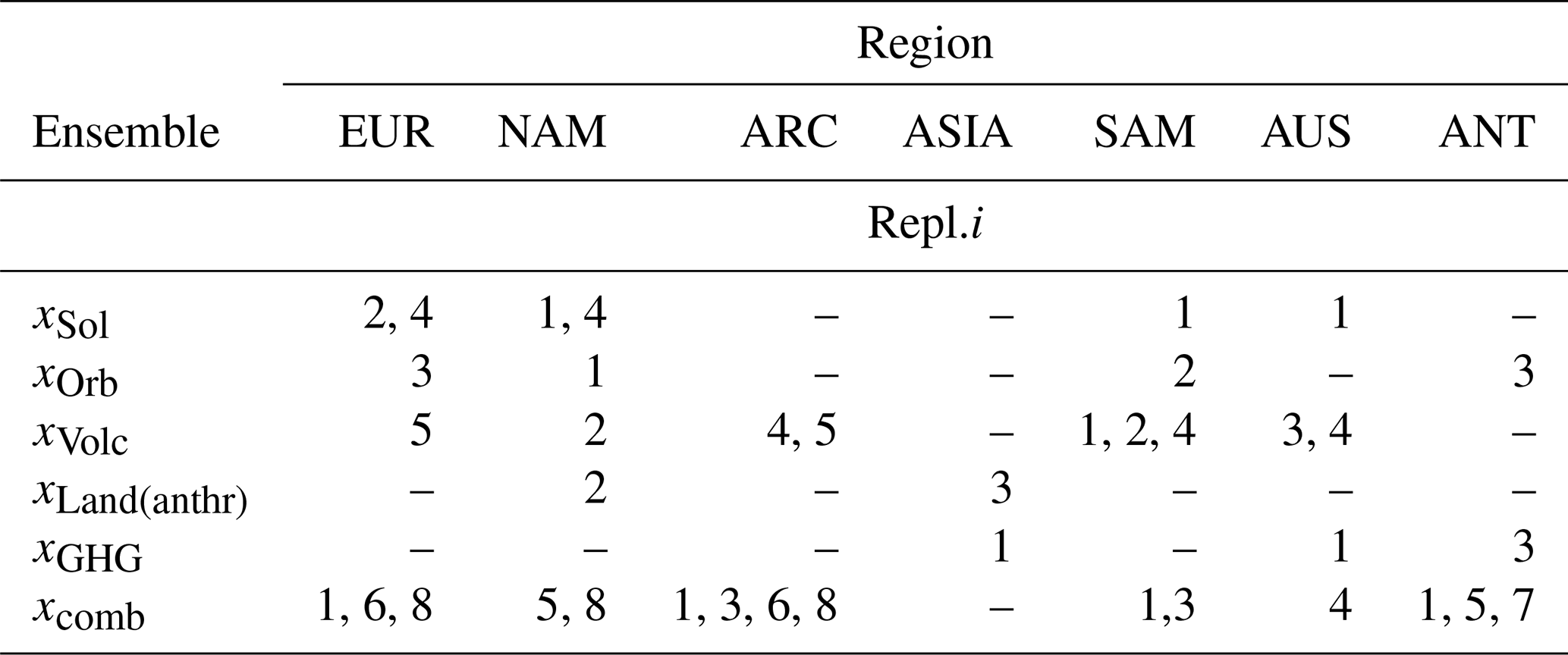
For our data, the application of model (4) indicated that some ensembles demonstrated at the significance level of 5 % an inconsistency with the assumptions associated with the CFA(k_𝚏,1) model in Eq. (4) and with estimator (3). To be able to proceed with our numerical experiment, some replicates from those problematic ensembles were eliminated. Table 1 provides an overview of the replicates eliminated.

Table 1 Overview of the replicates eliminated from the ensembles that do not satisfy the assumptions of estimator (3) and also of the CFA(k_𝚏,1) model.

2.2 Constructing data sets

Recall from the Introduction that, in our experiment, observational data are replaced by an appropriate climate model simulation. More precisely, such a climate model simulation is supposed to replace the true unobservable temperature, defined initially in SUN12. Combining the notations of LAS22 with the notations of SUN12, the mean-centred true temperature at time point t is modelled as follows:

$$\begin{array}{}\text{(5)}& {\mathit{\tau }}_t={\mathit{\xi }}_{\mathrm{ALL}t}^{\mathrm{T}}+{\mathit{\eta }}_{\mathrm{internal}t},\end{array}$$

where ${\mathit{\xi }}_{\mathrm{ALL}t}^{\mathrm{T}}$ is the true latent overall temperature response to all forcings, i.e. the forced component; and η_internal t is the internal random temperature variability of the real-world climate system, including any variability due to possible interactions between the forcings and internal processes.

Also, the forced and internal variability are regarded as mutually independent processes.

Among the climate model simulations presented earlier, the most suitable candidates for the role of pseudo τ are replicates of x_comb. Renaming x_{comb repl. it} in Eq. (1) as τ_{pseudo repl. it} and ${\stackrel{\mathrm{̃}}{\mathit{\delta }}}_{\mathrm{comb}\mathrm{repl}.it}$ as η_{internal pseudo repl. it} leads to

$$\begin{array}{}\text{(6)}& {\mathit{\tau }}_{\mathrm{pseudo}\mathrm{repl}.it}={\mathit{\xi }}_{\mathrm{comb}t}^{\mathrm{S}}+{\mathit{\eta }}_{\mathrm{internal}\mathrm{pseudo}\mathrm{repl}.it}.\end{array}$$

Choosing one replicate at a time enables us to construct the corresponding number of data sets. Fitting the statistical models to each of them makes it possible to investigate the stability of the performance of each statistical model of interest.

This is especially important when respecifications of the models by deleting and/or adding some hypothesised relations are performed. Although respecifications are supposed to be motivated from the climatological viewpoint, they are in essence results of a purely data-driven process. Therefore, it is crucial to apply some form of cross-validation with respect to the set of models considered in a sequence of model evaluations. The availability of additional data sets provides such an opportunity.

However, letting x_{comb repl.i}, $i=\mathrm{1},\mathrm{2},\mathrm{\dots },k_{\mathrm{comb}}$, be τ_pseudo, while all the remaining replicates are used for constructing the mean sequence ${\stackrel{\mathrm{‾}}{x}}_{\mathrm{comb}}$ amounts to creating data sets containing exactly identical information. This is expected to lead to (highly) correlated parameter estimates, which in turn may lead to misleading conclusions about the stability of the estimation procedure.

Table 2 Overview of the replicates of each x_𝚏, used to construct eight regional North America data sets (annual-mean temperature). Each data set contains different ${\stackrel{\mathrm{‾}}{x}}_{\mathrm{comb}}$ and τ_pseudo, where ${\stackrel{\mathrm{‾}}{x}}_{\mathrm{comb}}$ is constructed by averaging over four replicates randomly selected from the seven that remained after x_{comb repl.5} and x_{comb repl.8} had been eliminated (see Table 1) and after one of x_{comb repl.i}:s, $i=\mathrm{1},\mathrm{2},\mathrm{3},\mathrm{4},\mathrm{6},\mathrm{7},\mathrm{9},\mathrm{10}$, is chosen to represent τ, i.e. τ_pseudo.

To avoid this situation, the x_{comb repl.i}:s are arranged randomly into different data sets such that only some of them are used for constructing ${\stackrel{\mathrm{‾}}{x}}_{\mathrm{comb}}$. Table 2 provides an example of our way of reasoning for the data from the region of North America. Data sets for the remaining six regions are given in the Supplement (Sect. S1) along with the associated final statistical models.

3 Statistical models

In order to avoid excessive notations, from now on we will use neither the bar notation for mean sequences, nor the tilde for standardised latent variables. One can easily recognise models with standardised latent variables through the correlation matrices for their latent variables, while models with unstandardised latent variables are associated with variance–covariance matrices.

Another important aspect to point out is that CFA and SEM models presented in this section are adjusted for the use within a pseudo-proxy experiment. The adjustment is needed because the framework of LAS22 models common latent structures for simulated and observational data in terms of true latent temperature responses to real-world forcings. However, within a pseudo-proxy experiment, where observational data are replaced by climate model simulations, these true latent temperature responses are replaced by their simulated counterparts. The consequences of this replacement are as follows:

• The hypothesis of consistency between simulated and observed climate change is correct.

• The structure of the unforced components in the resulting statistical models is simpler compared to that associated with the original statistical models of LAS22.

It should also be realised that the correctness of the hypothesis of consistency is also applied to the ME model used in D&A studies, although the statistical framework of “optimal fingerprinting” models common latent structures for simulated and observational data in terms of simulated temperature responses to reconstructed forcings.

Model 1: the ME-CFA(6, 5) model

The ME-CFA(6, 5) model is given in Table 3. As indicated by its name, this is a CFA model derived from a measurement error (ME) regression model or, more precisely, from the ME model used in D&A studies. Its original form, with the notations adjusted to fit the present pseudo-proxy experiment, is given as follows:

$$\begin{array}{}\text{(7)}& {\mathit{\tau }}_{\mathrm{pseudo}t}=\sum _{\mathtt{\text{f}}}{\mathit{\beta }}_{\mathtt{\text{f}}}\cdot (x_{\mathtt{\text{f}}t}-{\stackrel{\mathrm{̃}}{\mathit{\delta }}}_{\mathtt{\text{f}}t})+{\mathit{\eta }}_{\mathrm{internal}\mathrm{pseudo}t},\end{array}$$

where f ∈{Sol, Orb, Volc, Land (anthr), GHG}, and t=1, 2, …,100.

Table 3 Parameters of Model 1, abbr. ME-CFA(6, 5) model, with six indicators and five standardised latent common factors with 1 degree of freedom.

^∗ The parameter assumed to be known a priori.

Within the ME-CFA(6, 5) model, all specific factors ${\stackrel{\mathrm{̃}}{\mathit{\delta }}}_{\mathtt{\text{f}}}$ are assumed to be both mutually independent and independent of the standardised common factors ${\mathit{\xi }}_{\mathtt{\text{f}}}^{\mathrm{S}}$. The same assumptions apply to the original ME model, but in contrast to the ME-CFA(6, 5) model, the former treats the latent temperature responses as unstandardised, each of which has its own variance ${\mathit{\sigma }}_{{\stackrel{\mathrm{̃}}{\mathit{\delta }}}_{\mathtt{\text{f}}}}^{\mathrm{2}}$. Under both representations, all ${\mathit{\xi }}_{\mathtt{\text{f}}}^{\mathrm{S}}$ factors are allowed to be correlated.

To arrive at the ME-CFA(6, 5) model, the ME model was first rewritten in a matrix form as shown in Table 4.

Table 4 The ME model from Eq. (7) with the associated variance–covariance matrix for the latent variables, written in a matrix form.

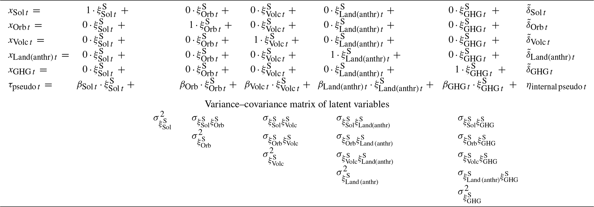
Here, the ME model appears as a factor model with unstandardised latent factors. Their subsequent standardisation gives the ME-CFA(6, 5) model, whose factor loadings are related to the parameters of the ME model as follows: Ssim $={\mathit{\sigma }}_{{\mathit{\xi }}_{\mathrm{Sol}}^{\mathrm{S}}}$, Strue $={\mathit{\beta }}_{\mathrm{Sol}}\cdot {\mathit{\sigma }}_{{\mathit{\xi }}_{\mathrm{Sol}}^{\mathrm{S}}}$, Osim $={\mathit{\sigma }}_{{\mathit{\xi }}_{\mathrm{Orb}}^{\mathrm{S}}}$, Otrue $={\mathit{\beta }}_{\mathrm{Orb}}\cdot {\mathit{\sigma }}_{{\mathit{\xi }}_{\mathrm{Orb}}^{\mathrm{S}}}$, etc. These links between the models' parameters show the following:

• The hypothesis H₀: β_𝚏=0 tested at the detection stage in D&A studies concerns true loadings under the ME-CFA(6, 5) model; for example, H₀: β_Sol=0 corresponds to H₀: Strue =0.

• The hypothesis of consistency H₀: β_𝚏=1 tested at the attribution stage in D&A studies concerns the ratios between true and sim loadings under the ME-CFA(6, 5) model; for example, H₀: β_Sol=1 corresponds to H₀: Strue $/$ Ssim =1.

Thus, as was found in LAS22, the questions posed in D&A studies can also be addressed using CFA models in place of the ME model specification. The present numerical experiment gives us an opportunity not only to evaluate the performance of the ME model used in D&A studies when it is applied to the same data as the CFA and SEM models of interest, but also to demonstrate in practice the way of analysing the ME model when it is rewritten as a CFA model. Such a practical example may also facilitate the understanding of the transition from the ME model specification to more complex CFA and SEM models, constituting the core of LAS22.

It should also be noted that the ideas of CFA make it possible to test the hypothesis of consistency without performing multiple simultaneous tests concerning the above-defined ratios. One simply fits the ME-CFA(6, 5) model to data under the restrictions Strue=Ssim, Otrue=Osim, etc. However, this implies that one cannot use the same estimator as that used in D&A studies, namely the total least squares (TLS) estimator.

To evaluate the performance of the ME model used in D&A studies, we fit the ME-CFA(6, 5) model as if it were a ME model associated with the TLS estimator. That is, the parameter estimates will be obtained under the assumption that the whole error variance–covariance matrix is known a priori, as shown in Table 3. Under this assumption, the model is over-identified with 1 degree of freedom, which permits model validity to be checked. To calculate the degrees of freedom, one subtracts the total number of free parameters (20) from the number of unique equations in the variance–covariance matrix of the observed indicators (21).

For checking purposes, we nevertheless use the principles of CFA to their full extent (see Sect. S2.4 in the Supplement), instead of using the methods developed specifically for ME models (see, for example, Fuller, 1987)

As a final comment, let us emphasise that since the hypothesis of consistency is correct, all β_𝚏 coefficients in the ME model are equal to 1, and the sim coefficients in the ME-CFA(6, 5) model are equal to their corresponding true coefficients; for example, Ssim=Strue. So, if the underlying structure of data is consistent with the structure defined by the ME-CFA(6, 5) model, then its fit to data is expected to be adequate, and the estimates are expected to be admissible, provided, of course, all temperature responses are detected; that is, the hypothesis H₀: β_𝚏=0 is rejected for each f. If not, the underlying latent structure needs to be respecified accordingly, which, however, means that we have to move to the CFA model suggested within the LAS22 framework (see the next section).

Model 2: the confirmatory factor analysis (CFA) model

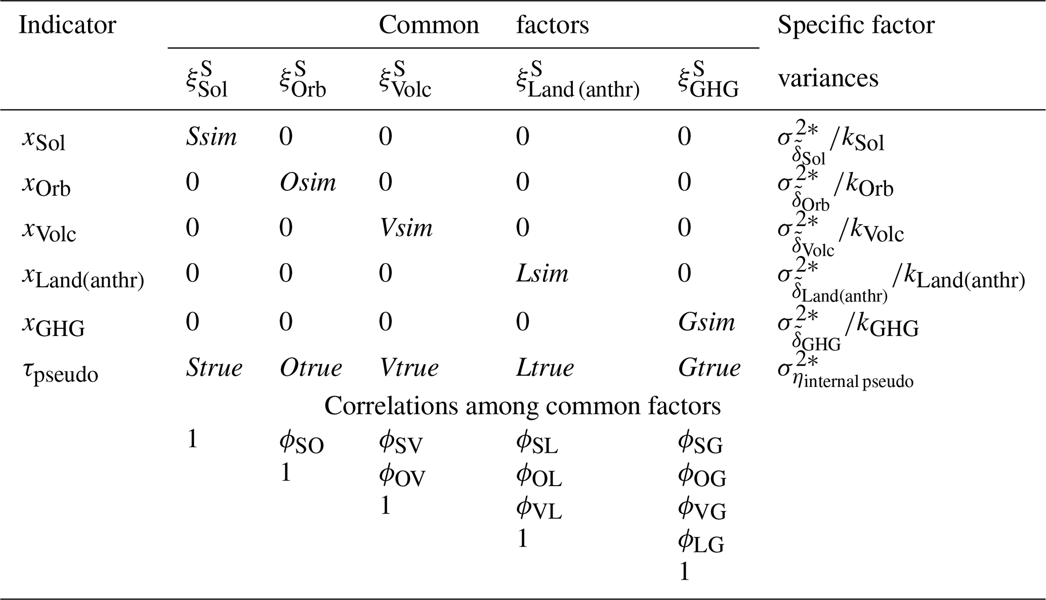
Model 2 is formulated by extending the ME-CFA(6, 5) model both in terms of the number of indicators and in terms of common latent factors. The parameters of the resulting model, abbr. the CFA(7, 6) model, are presented in Table 5.

Table 5 Parameters of Model 2, abbr. CFA(7, 6), containing seven indicators and six standardised latent factors with 12 degrees of freedom.

^∗ The parameter assumed to be known a priori.

As one can see, adding x_comb as an additional indicator makes it possible to introduce the interaction term, which denotes the deviation from the additivity of the forcing effects. In this statistical model, ξ_interact is interpreted as an overall temperature response to all possible interactions between the forcings under consideration. As a result, ξ_interact in this model is both of natural and anthropogenic character. To test the hypothesis that the effect of interactions on the temperature is negligible, one estimates this factor model under the restrictions that Isim and all associated correlations, i.e. ${\mathit{\varphi }}_{\mathrm{SI}},\mathrm{\dots },{\mathit{\varphi }}_{\mathrm{GI}}$, are zero.

Further, as follows from the correlation matrix for the common factors, the CFA(7, 6) model hypothesises the mutual uncorrelatedness between ${\mathit{\xi }}_{\mathrm{Sol}}^{\mathrm{S}}$, ${\mathit{\xi }}_{\mathrm{Orb}}^{\mathrm{S}}$, ${\mathit{\xi }}_{\mathrm{Volc}}^{\mathrm{S}}$, and ${\mathit{\xi }}_{\mathrm{Land}\left(\mathrm{anthr}\right)}^{\mathrm{S}}$. This hypothesis was motivated by the substantive knowledge about the underlying forcings that are acting on different timescales and with different character of their temporal evolutions. This makes it reasonable to expect different shapes, i.e. temporal patterns, of the temperature responses caused by them.

On the other hand, it is difficult to hypothesise zero correlations between ${\mathit{\xi }}_{\mathrm{interact}}^{\mathrm{S}}$ and ${\mathit{\xi }}_{\mathrm{Sol}}^{\mathrm{S}}$,  ${\mathit{\xi }}_{\mathrm{Orb}}^{\mathrm{S}}$, ${\mathit{\xi }}_{\mathrm{Volc}}^{\mathrm{S}}$, and ${\mathit{\xi }}_{\mathrm{Land}\left(\mathrm{anthr}\right)}^{\mathrm{S}}$. Thus, the correlation coefficients ϕ_SI, ϕ_OI, ϕ_VI, and ϕ_LI are treated as unknown parameters to be estimated, provided Isim is not set to zero.

Another difference between the ME-CFA(6, 5) model and the CFA(7, 6) model is that the ME-CFA(6, 5) model treats ${\mathit{\sigma }}_{{\mathit{\eta }}_{\mathrm{internal}\mathrm{pseudo}}}^{\mathrm{2}}$ as an a priori known parameter, while the CFA(7, 6) model treats this parameter as unknown. In real-world analyses, where observational data are not replaced by τ_pseudo, the latter approach allows us to take into account not only the internal temperature variability, but also a non-climatic noise embedded in proxy data, which is a part of observational data. Typically, the variability of such non-climatic noise is assumed to be large (Hegerl et al., 2007; Jones et al., 2009).

Another aspect, worthy of discussion, is the ability of the CFA model presented to discriminate between the natural and anthropogenic components of ${\mathit{\xi }}_{\mathrm{GHG}}^{\mathrm{S}}$. Since common factors within the CFA model specification can be related to each other only through correlations, the only way to get some indication of the importance of ${\mathit{\xi }}_{\mathrm{GHG}\left(\mathrm{anthr}\right)}^{\mathrm{S}}$ and ${\mathit{\xi }}_{\mathrm{GHG}\left(\mathrm{natur}\right)}^{\mathrm{S}}$ is to study the significance of the estimates of the correlations relating ${\mathit{\xi }}_{\mathrm{GHG}}^{\mathrm{S}}$ to other temperature responses. For example, a strong estimate of ϕ_LG, presupposed to relate ${\mathit{\xi }}_{\mathrm{GHG}\left(\mathrm{anthr}\right)}^{\mathrm{S}}$ to ${\mathit{\xi }}_{\mathrm{Land}\left(\mathrm{anthr}\right)}^{\mathrm{S}}$ due to their common source that is human activity, makes it justified to describe the effect of the anthropogenic changes in the GHG forcing as well pronounced. Further, any significant estimate of ϕ_SG, ϕ_OG, or ϕ_VG, presupposed to relate ${\mathit{\xi }}_{\mathrm{Sol}}^{\mathrm{S}}$, ${\mathit{\xi }}_{\mathrm{Orb}}^{\mathrm{S}}$, and ${\mathit{\xi }}_{\mathrm{Volc}}^{\mathrm{S}}$, respectively, to ${\mathit{\xi }}_{\mathrm{GHG}\left(\mathrm{natur}\right)}^{\mathrm{S}}$ gives an indication that the natural component of ${\mathit{\xi }}_{\mathrm{GHG}}^{\mathrm{S}}$ is detected as well. Concerning the correlations relating the interaction term to ${\mathit{\xi }}_{\mathrm{GHG}}^{\mathrm{S}}$, it is unfortunately difficult to provide an interpretation of their significance due to the mixed nature of the interaction term under the CFA model specification.

Finally, it can be seen in Table 5 that the CFA model takes into account the correctness of the hypothesis of consistency motivated by the properties of the pseudo-proxy experiment. This is reflected by the fact that each ${\mathit{\xi }}_{\mathtt{\text{f}}}^{\mathrm{S}}$ has the same factor loading on τ_pseudo and x_comb and on the corresponding x_𝚏. Thus, the total number of the free parameters that are to be estimated is 16. Since there are 28 unique equations in the variance–covariance matrix of the observed indicators, it implies that the model has 12 degrees of freedom.

Just as in the case of the ME-CFA(6, 5) model, the correctness of the hypothesis of consistency means that an inadequate model fit to the data and/or inadmissible estimates are due to a misspecified latent structure. Respecifications of the structure, requiring the introduction of causal inputs, entails in turn the movement to the SEM specifications, suggested within the LAS22 framework (see the next section). If some modified version of the CFA model presented results in a climatologically defensible solution and fits adequately to the data, then it is a motivation to accept this CFA model as a reasonable approximation of the underlying latent structure.

Model 3: the structural equation modelling (SEM) model

The SEM model analysed in this experiment is presented graphically in Fig. 1. This SEM model is a modified version of the basic SEM model suggested by LAS22. The modification is performed in order to take into account the properties of the x_{Land (anthr)} climate model simulations, forced only by the anthropogenic land-use forcing.

Just like the CFA(7, 6) model in Table 5, the SEM model takes into account that the hypothesis of consistency within a pseudo-proxy experiment is correct and that the variances of the ${\stackrel{\mathrm{̃}}{\mathit{\delta }}}_{\mathtt{\text{f}}}$ factors are known a priori, while the variance of η_{internal pseudo} is an unknown model parameter.

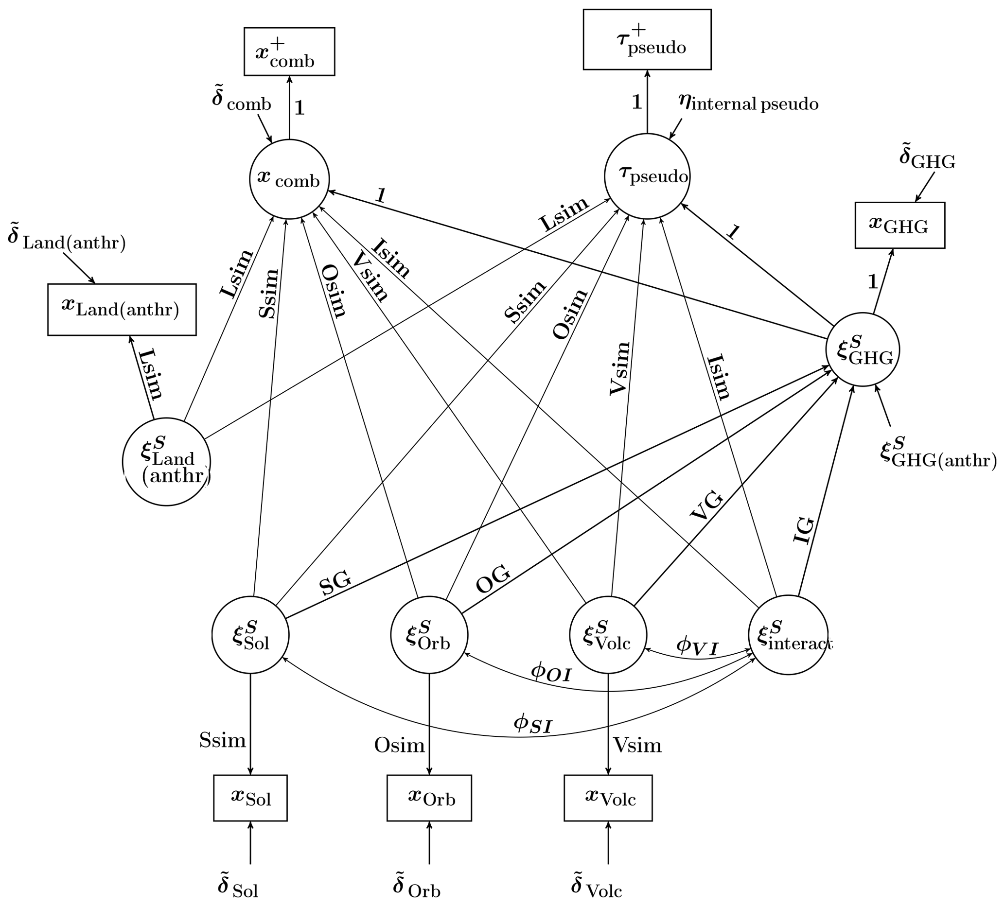
Figure 1 Path diagram for the SEM model with five standardised exogenous latent factors, ${\mathit{\xi }}_{\mathrm{Sol}}^{\mathrm{S}}$,  ${\mathit{\xi }}_{\mathrm{Orb}}^{\mathrm{S}}$, ${\mathit{\xi }}_{\mathrm{Volc}}^{\mathrm{S}}$, ${\mathit{\xi }}_{\mathrm{Land}\left(\mathrm{anthr}\right)}^{\mathrm{S}}$, and  ${\mathit{\xi }}_{\mathrm{interact}}^{\mathrm{S}}$, and one endogenous latent factor, ${\mathit{\xi }}_{\mathrm{GHG}}^{\mathrm{S}}$. The model has 14 degrees of freedom.

In contrast to the CFA(7, 6) model, the SEM model reflects the substantive knowledge of atmosphere–climate interactions, which may arise when natural changes in the levels of GHG in the atmosphere are caused by other climatic processes of natural origin. In the SEM model, this is reflected through the causal inputs received by ${\mathit{\xi }}_{\mathrm{GHG}}^{\mathrm{S}}$ or more precisely by its natural component. The inputs come from ${\mathit{\xi }}_{\mathrm{Sol}}^{\mathrm{S}}$,  ${\mathit{\xi }}_{\mathrm{Orb}}^{\mathrm{S}}$,  ${\mathit{\xi }}_{\mathrm{Volc}}^{\mathrm{S}}$, and ${\mathit{\xi }}_{\mathrm{interact}}^{\mathrm{S}}$, which leads to the following equation for ${\mathit{\xi }}_{\mathrm{GHG}\mathrm{t}}^{\mathrm{S}}$:

$$\begin{array}{}\text{(8)}& \begin{array}{rl}{\mathit{\xi }}_{\mathrm{GHG}t}^{\mathrm{S}}& ={\mathit{\xi }}_{\mathrm{GHG}\left(\mathrm{natur}\right)t}^{\mathrm{S}}+{\mathit{\xi }}_{\mathrm{GHG}\left(\mathrm{anthr}\right)t}^{\mathrm{S}}=\mathit{\text{SG}}\cdot {\mathit{\xi }}_{\mathrm{Sol}t}^{\mathrm{S}}+\mathit{\text{OG}}\cdot {\mathit{\xi }}_{\mathrm{Orb}t}^{\mathrm{S}}\\ & +\mathit{\text{VG}}\cdot {\mathit{\xi }}_{\mathrm{Volc}t}^{\mathrm{S}}+\mathit{\text{IG}}\cdot {\mathit{\xi }}_{\mathrm{interact}t}^{\mathrm{S}}++{\mathit{\xi }}_{\mathrm{GHG}\left(\mathrm{anthr}\right)t}^{\mathrm{S}}.\end{array}\end{array}$$

Concerning the interaction term in Eq. (8), it should be noted that ${\mathit{\xi }}_{\mathrm{interact}t}^{\mathrm{S}}$ under the SEM specification is interpreted as the overall effect of all possible interactions between physically independent processes acting simultaneously in the climate system. That is, ${\mathit{\xi }}_{\mathrm{interact}t}^{\mathrm{S}}$ in the SEM model presented represents the overall effect of the interactions between the natural forcings and anthropogenic changes in land-use and GHG forcings. Consequently, ${\mathit{\xi }}_{\mathrm{interact}t}^{\mathrm{S}}$ does not have a pure natural character as we would like.

Unfortunately, with the available climate model simulations in hand, it is not possible to model the natural component of ${\mathit{\xi }}_{\mathrm{interact}t}^{\mathrm{S}}$ separately from the anthropogenic one. For this, one needs two types of climate model simulations, one forced by the combination of the natural forcings and one by the combination of anthropogenic forcings.

The interpretation issue of ${\mathit{\xi }}_{\mathrm{interact}t}^{\mathrm{S}}$ highly motivates us to fit first the SEM model under the hypothesis of additivity, which corresponds to setting Isim and all correlations associated with the interaction term to zero.

The absence of climate model simulations forced only by the anthropogenic changes in the GHG forcings also makes it impossible to model the anthropogenic component of ${\mathit{\xi }}_{\mathrm{GHG}}^{\mathrm{S}}$ as an individual latent factor. Instead, ${\mathit{\xi }}_{\mathrm{GHG}\left(\mathrm{anthr}\right)}^{\mathrm{S}}$ is separated from ${\mathit{\xi }}_{\mathrm{GHG}\left(\mathrm{natur}\right)}^{\mathrm{S}}$ only by modelling it as a disturbance term contributing to the variability of ${\mathit{\xi }}_{\mathrm{GHG}}^{\mathrm{S}}$ randomly. In case both natural and anthropogenic components are detected, this modelling approach does not allow us to assess the direct contribution of anthropogenic changes in the GHG forcing to the temperature variability. Nevertheless, separating these components allows us to see their contributions more clearly compared to the approach of the CFA model, where these two components cannot be separated in any way. In case no causal paths to ${\mathit{\xi }}_{\mathrm{GHG}}^{\mathrm{S}}$ are detected, then ${\mathit{\xi }}_{\mathrm{GHG}}^{\mathrm{S}}$ is to be replaced by ${\mathit{\xi }}_{\mathrm{GHG}\left(\mathrm{anthr}\right)}^{\mathrm{S}}$, which makes it possible to model it as a separate latent factor just as ${\mathit{\xi }}_{\mathrm{Land}\left(\mathrm{anthr}\right)}^{\mathrm{S}}$ is modelled.

Like the CFA(7, 6) model, the SEM model in Fig. 1 can be modified in various ways. For example, the causal inputs from ${\mathit{\xi }}_{\mathrm{Sol}}^{\mathrm{S}}$,  ${\mathit{\xi }}_{\mathrm{Orb}}^{\mathrm{S}}$,  ${\mathit{\xi }}_{\mathrm{Volc}}^{\mathrm{S}}$, and ${\mathit{\xi }}_{\mathrm{interact}}^{\mathrm{S}}$ to ${\mathit{\xi }}_{\mathrm{GHG}}^{\mathrm{S}}$ can be replaced (or complemented) by the causal inputs from x_comb and/or τ_pseudo (and/or from x_GHG). These inputs can be taken as an indication that the temperature sequences analysed may contain a certain effect of subsequent changes in the GHG forcing, caused by the changed climate itself, and that might be reflected in the reconstruction of the GHG forcing, used to drive the climate model under study. Note that this effect may be insignificant, but freeing up these paths can be important for achieving a good overall model fit to the data and/or the stability of the estimation process.

Analogously, we may allow ${\mathit{\xi }}_{\mathrm{GHG}}^{\mathrm{S}}$ to receive inputs from x_Sol, x_Orb, and/or x_Volc. Note that the CFA specification does not allow observed indicators to influence latent factors. The identifiability status of each modified SEM model should be determined on a case-by-case basis.

According to LAS22, ${\mathit{\xi }}_{\mathrm{GHG}}^{\mathrm{S}}$ under the SEM model is an endogenous variable, receiving causal inputs. Therefore, its variance is not a model parameter, which can be estimated when the model is fitted to the data. However, it can be calculated afterwards. This is important because knowledge about this variance is crucial when gauging the direct overall effect of the GHG forcing on the temperature relative to the other forcings. Indeed, by taking the square root of $\widehat{\text{Var}}\left({\mathit{\xi }}_{\mathrm{GHG}}^{\mathrm{S}}\right)$, we obtain the estimate of the standardised coefficient for ${\mathit{\xi }}_{\mathrm{GHG}}^{\mathrm{S}}$ that is to be compared to $\widehat{\mathit{Ssim}}$, $\widehat{\mathit{Osim}}$, $\widehat{\mathit{Vsim}}$, $\widehat{\mathit{Lsim}}$, and $\widehat{\mathit{Isim}}$ (when they are available).

Statistical significance of this estimate, which we denote ${\widehat{\mathit{Gsim}}}_{\mathit{SEM}}$, can be judged from the statistical significance, i.e. two-sided p value, of $\widehat{\text{Var}}\left({\mathit{\xi }}_{\mathrm{GHG}}^{\mathrm{S}}\right)$. For example, rejecting H₀: $\text{Var}\left({\mathit{\xi }}_{\mathrm{GHG}}^{\mathrm{S}}\right)=\mathrm{0}$ at the α significance level corresponds to rejecting H₀: Gsim${}_{\mathit{SEM}}=\sqrt{\text{Var}\left({\mathit{\xi }}_{\mathrm{GHG}}^{\mathrm{S}}\right)}=\mathrm{0}$ at the same significance level. Given admissible estimates of all parameters, and provided that ${\mathit{\xi }}_{\mathrm{GHG}}^{\mathrm{S}}$ receives causal inputs, one can calculate $\text{Var}\left({\mathit{\xi }}_{\mathrm{GHG}}^{\mathrm{S}}\right)$ as follows:

1. Derive the theoretical expression for $\text{Var}\left({\mathit{\xi }}_{\mathrm{GHG}}^{\mathrm{S}}\right)$ as a function of the model parameters in accordance with Eq. (S13), given in Sect. S2.2 in the Supplement.

2. Replace unknown free parameters in $\text{Var}\left({\mathit{\xi }}_{\mathrm{GHG}}^{\mathrm{S}}\right)$ by their estimates to obtain $\widehat{\text{Var}}\left({\mathit{\xi }}_{\mathrm{GHG}}^{\mathrm{S}}\right)$.

3. Apply the delta method, described in Sect. S2.5 in the Supplement, to obtain an estimate of the variance of the asymptotic distribution of $\widehat{\text{Var}}\left({\mathit{\xi }}_{\mathrm{GHG}}^{\mathrm{S}}\right)$.

4. Calculate the two-sided p value for $\widehat{\text{Var}}\left({\mathit{\xi }}_{\mathrm{GHG}}^{\mathrm{S}}\right)$ using the fact that under the null hypothesis H₀: $\text{Var}\left({\mathit{\xi }}_{\mathrm{GHG}}^{\mathrm{S}}\right)=\mathrm{0}$, the test statistic $\widehat{\text{Var}}\left({\mathit{\xi }}_{\mathrm{GHG}}^{\mathrm{S}}\right)/\sqrt{\widehat{\text{Var}}\left(\widehat{\text{Var}}\right({\mathit{\xi }}_{\mathrm{GHG}}^{\mathrm{S}}\left)\right)}$ is approximately normally distributed with zero mean and a variance of 1. One can also calculate an approximate confidence interval using Eq. (S25), given in the Supplement, which, however, was not done here due to space constraints.

4 Numerical results

To avoid an excessively long result section, we present a detailed discussion and interpretation of the results only for one of the regions, namely for North America (see Sect. 4.1). This choice of region is arbitrary. A similar detailed presentation and interpretation of results for the remaining six regions is provided in the Supplement. A brief overview of the results for all seven regions is presented in Sect. 4.2.

4.1 Numerical results: the North America data (annual-mean temperature)

The structure of this section is the following. First, we present the results of the preliminary analysis of each (final) single-forcing ensemble, given in Table 2, by means of the CFA(k_𝚏,1) model, defined in Eq. (4). At this stage, we also discuss some results of estimating the variance of the internal temperature variability, denoted ${\mathit{\sigma }}_{{\stackrel{\mathrm{̃}}{\mathit{\delta }}}_{\mathtt{\text{f}}}}^{\mathrm{2}}$, by means of estimator (3). Further, we present in turn the results of fitting the three statistical models of interest, followed by a summary and conclusions.

4.1.1 Preliminary analysis of the single-forcing ensembles by means of the CFA(k_𝚏,1) model

As a preliminary step, we apply the CFA(k_𝚏,1) model to the single-forcing ensembles in order to get a preliminary idea about the magnitude of the forcing effects. The estimates of α_𝚏, provided by the CFA(k_𝚏,1) model, can be useful for judging the appropriateness of the estimates provided by the large CFA and SEM models of interest. Importantly, the ensembles have already been screened (and reduced when it was needed), meaning that the CFA(k_𝚏,1) model fits each ensemble adequately, which in turn increases the reliability of the parameter estimates obtained.

The analysis of the x_{Land (anthr)} ensemble indicated that the effect of the reconstructed land-use forcing is not detected (at the 5 % significance level) in the simulated annual-mean temperature in North America during the period of 850–1849 CE (${\widehat{\mathit{\alpha }}}_{\mathrm{Land}\left(\mathrm{anthr}\right)}=\mathrm{0.039}$, p value =0.13)². This conclusion seems to be in concert with the temporal evolution of the land-use forcing, which shows quite modest variations over North America during the analysis period (see Fig. S4.5 in Fetisova et al., 2017).

Similar analyses of the x_Sol, x_Volc, and x_GHG ensembles suggested that the effect of the corresponding forcings is well pronounced in the simulated annual-mean temperature in North America during the period of 850–1849 CE: ${\widehat{\mathit{\alpha }}}_{\mathrm{Sol}}=\mathrm{0.049}$ (p value =6.2e–03), ${\widehat{\mathit{\alpha }}}_{\mathrm{Volc}}=\mathrm{0.132}$ (p value =2.0e–29), and ${\widehat{\mathit{\alpha }}}_{\mathrm{GHG}}=\mathrm{0.051}$ (p value =1.0e–04).

For each of the above-mentioned ensembles, an a priori estimate of ${\mathit{\sigma }}_{{\stackrel{\mathrm{̃}}{\mathit{\delta }}}_{\mathtt{\text{f}}}}^{\mathrm{2}}$ was also derived by means of estimator (3). All estimates derived were found to be (approximately) equal to the corresponding estimates provided by the CFA(k_𝚏,1) model.

An opposite result was observed for the x_Orb ensemble. The estimate of ${\mathit{\sigma }}_{{\stackrel{\mathrm{̃}}{\mathit{\delta }}}_{\mathrm{Orb}}}^{\mathrm{2}}/\mathrm{2}$, where ${\mathit{\sigma }}_{{\stackrel{\mathrm{̃}}{\mathit{\delta }}}_{\mathrm{Orb}}}^{\mathrm{2}}$ was provided by estimator (3), turned out to be larger than the sample variance of the mean sequence x_Orb. A natural interpretation of this result is that the effect of the orbital forcing on the simulated annual-mean temperature in North America during the period of 850–1849 CE is non-detectable. The conclusion was supported by (i) the fact that only the CFA(k_𝚏,0) model could be fitted to the x_Orb ensemble, while the estimation procedure of the CFA(k_𝚏,1) model failed to converge to a solution, and by (ii) the temporal evolution of the orbital forcing, which shows virtually no change over North America on an annual average basis during the analysis period (see Fig. S4.3 in Fetisova et al., 2017). To make the estimation of our large statistical models meaningful, ${\mathit{\sigma }}_{{\stackrel{\mathrm{̃}}{\mathit{\delta }}}_{\mathrm{Orb}}}^{\mathrm{2}}/\mathrm{2}$ was set to the sample variance of the mean sequence x_Orb, which requires setting the parameter Osim to zero.

4.1.2 Results of estimating Model 1, i.e. the ME-CFA(6, 5) model

Due to treating correlations among the latent factors as free parameters, the ME-CFA(6, 5) model (and the ME model as well) becomes theoretically under-identified, if at least one of the factor loadings is restricted a priori to zero, while the associated correlations are still treated as free parameters. In practice, the data, for which some factor loadings are expected to be arbitrarily near zero, are associated with the so-called weak-signal regime (DelSole et al., 2019). This regime entails so-called “empirical under-identifiability”, characterised by inadmissible solutions, or very wide confidence intervals, or the failure of the estimation procedure to converge to a solution.

Therefore, knowing that fitting the ME-CFA(6, 5) model to the North America data is likely to result in negligible estimates of Osim and Lsim, it is reasonable to expect different consequences of the under-identifiability. As we see in Table 6, this is the case. For two of the eight data sets analysed, the estimation procedure failed to converge to a solution. The solution for the remaining data sets is inadmissible, which follows from the fact that the estimates of the correlation coefficients, associated with ${\mathit{\xi }}_{\mathrm{Orb}}^{\mathrm{S}}$ and ${\mathit{\xi }}_{\mathrm{Land}\left(\mathrm{anthr}\right)}^{\mathrm{S}}$, exceed their admissible range; that is, they are larger than 1 in absolute values.

Table 6 The result of estimating Model 1, i.e. the ME-CFA(6, 5) model, defined in Table 3. The estimates in bold font are inadmissible.

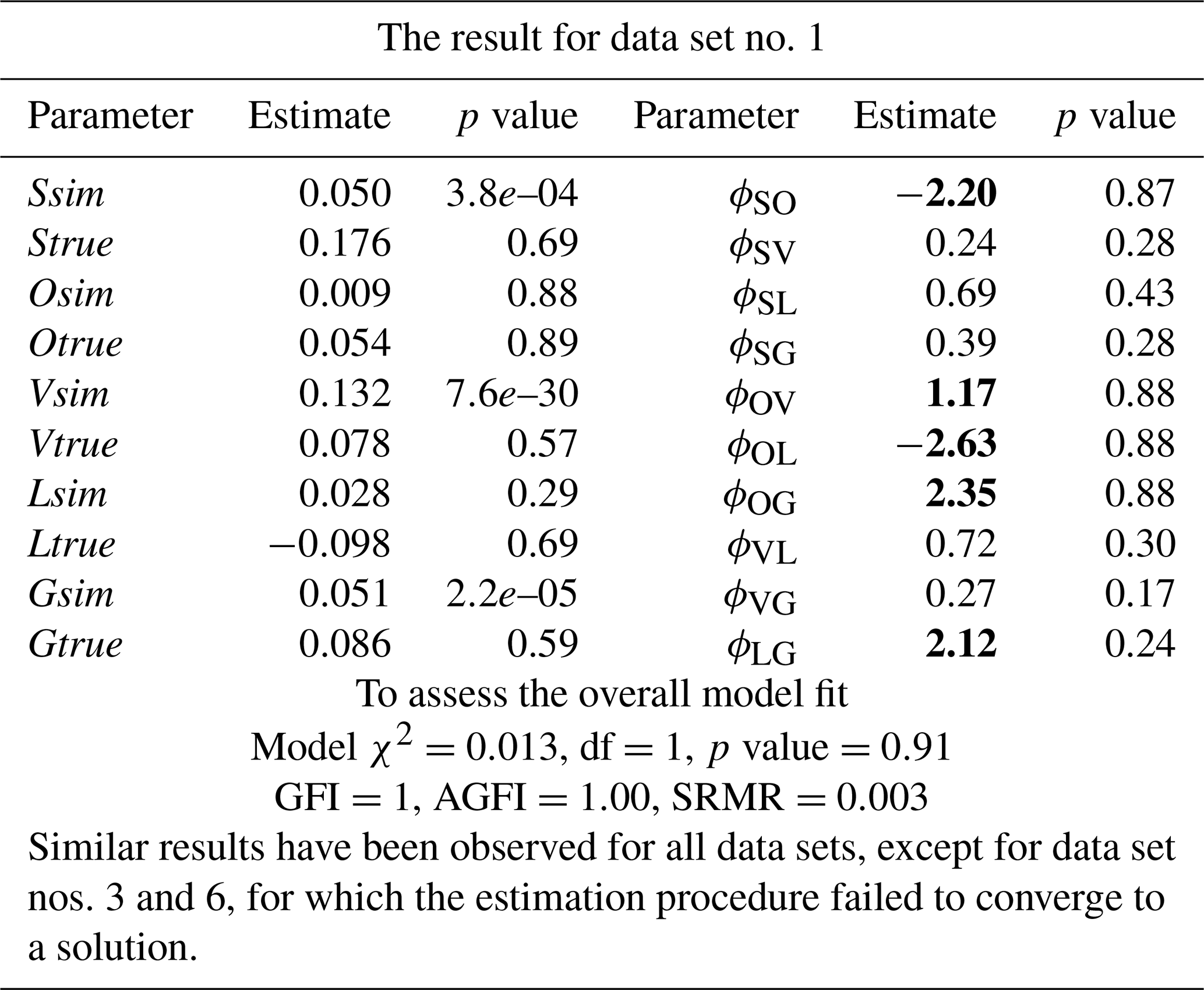
Based on this result, the ME-CFA(6, 5) model cannot be selected as an adequate approximation of the underlying latent relationships, even if the model fits the data perfectly, both statistically and heuristically (e.g. for data set no. 1, the p value associated with the χ² statistic is 0.91, which is larger than 0.05, and the observed values of the heuristic indices are within their acceptance areas: $\text{GFI}=\mathrm{1}>\mathrm{0.90}$, $\text{AGFI}=\mathrm{1}>\mathrm{0.80}$, and $\text{SRMR}=\mathrm{0.003}<\mathrm{0.08}$).

To avoid the weak-signal regime, we could delete x_Orb and x_{Land (anthr)} from the data set and modify the ME-CFA(6, 5) model accordingly. However, this approach does not guarantee that the correlation matrix of the remaining latent factors is non-singular and describes the latent relationships adequately. Moreover, in real-world analysis, such eliminations would prevent us from evaluating the eliminated climate model simulations against observational data. Therefore, LAS22 suggests moving to the CFA model specification, and, if necessary, further to the SEM specification to allow parameters to be set to zero in the course of the analysis.

4.1.3 Results of estimating Model 2, i.e. the CFA(7, 6) model

In order to avoid empirical under-identifiability, each modified version of the basic CFA(7, 6) model was formulated under the restrictions that Osim, Lsim, and all associated correlation coefficients are zero. Another positive consequence of these restrictions is the increased number of degrees of freedom.

The estimates of the modified version, which demonstrated the most stable performance across all data sets, are presented in Table 7. According to the table, the CFA model fits the data well both statistically and heuristically. For data set no. 1, to which the CFA model was initially fitted, the p value for the χ² statistic is 0.67, which is much larger than 0.05, and the observed heuristic indices are within their acceptance areas: $\text{GFI}=\mathrm{0.96}>\mathrm{0.9}$, $\text{AGFI}=\mathrm{0.93}>\mathrm{0.8}$, and $\text{SRMR}=\mathrm{0.065}<\mathrm{0.08}$. The average overall model fit is also good, especially in terms of the SRMR values (min(SRMR)=0.063, mean(SRMR)=0.065, and max(SRMR)=0.069).

Table 7 The result of estimating Model 2, i.e. the CFA(7, 6) model, defined in Table 5.

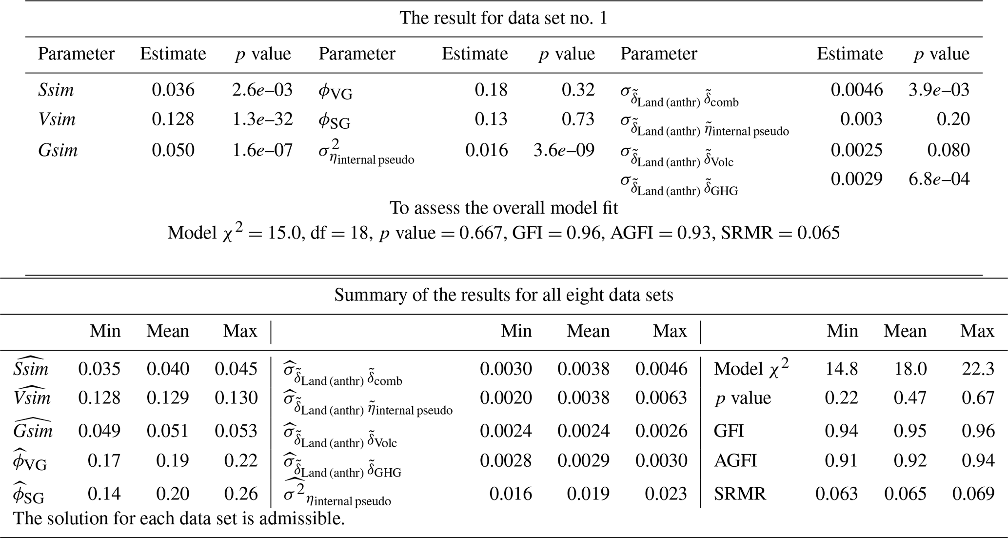
According to the parameter estimates, the CFA model suggests that the (direct) effects of the solar and volcanic forcings are well pronounced in the simulated annual-mean temperature in North America during 850–1849 CE. For example, for data set no. 1, it was observed that $\widehat{\mathit{Ssim}}=\mathrm{0.036}$ with p value=2.6e–03, and $\widehat{\mathit{Vsim}}=\mathrm{0.128}$ with p value=1.3e–32. This is in agreement with the corresponding preliminary conclusions provided by the CFA(k_𝚏, 1) model. Comparing $\widehat{\mathit{Ssim}}$ to $\widehat{\mathit{Vsim}}$, we may also say that the detected effect of the volcanic forcing is much stronger than the detected effect of the solar forcing.

The overall (direct) effect of the GHG forcing is also estimated by the CFA model as significant (for data set no. 1, $\widehat{\mathit{Gsim}}=\mathrm{0.050}$ with p value =1.6e–07). Further, the CFA model detects a weak relation of ${\mathit{\xi }}_{\mathrm{GHG}}^{\mathrm{S}}$ to ${\mathit{\xi }}_{\mathrm{Sol}}^{\mathrm{S}}$ and to ${\mathit{\xi }}_{\mathrm{Volc}}^{\mathrm{S}}$. For data set no. 1, the estimates of the corresponding correlation coefficients are ${\widehat{\mathit{\varphi }}}_{\mathrm{VG}}=\mathrm{0.18}$ (p value =0.32) and ${\widehat{\mathit{\varphi }}}_{\mathrm{SG}}=\mathrm{0.13}$ (p value =0.73). Together with the significant estimate of Gsim, this result suggests that the overall effect of the GHG forcing is mostly of anthropogenic character. Climatologically, the significant effect of anthropogenic changes in the reconstructed GHG forcing can be justified by an effect mainly in the last about 1 century of data in the analysed period. Hence, the CFA model presented not only has an acceptable fit and admissible solutions, but also seems to be climatologically interpretable. However, prior to drawing final conclusions, let us discuss the result of fitting the SEM model.

4.1.4 Results of estimating Model 3, i.e. the SEM model

When estimating the above-presented CFA model, the modification indices indicated that the overall model fit could be further improved if x_{Land (anthr)} received a causal input from x_Volc. Keeping in mind that x_{Land (anthr)} does not contain the forced component ${\mathit{\xi }}_{\mathrm{Land}\left(\mathrm{anthr}\right)}^{\mathrm{S}}$ due to the restriction Lsim=0, this input would co-relate both forced and internal temperature variability, generated by the x_Volc climate model, to the internal temperature variability, generated by the x_{Land (anthr)} climate model.

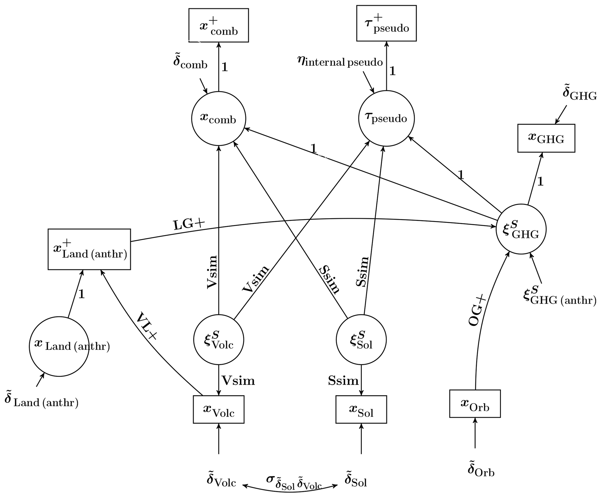
Figure 2 Path diagram of the modified version of the SEM model from Fig. 1 (region: North America).

Although no dynamical relationships between the reconstructions of the forcings and the internal processes were implemented in the climate modelling experiment under consideration, the causal input from x_Volc to x_{Land (anthr)}, nevertheless, would statistically express more complicated climatological processes, which may occur in the real-world climate system and which may be reflected both in the forcing reconstructions and in the physical basis for the internal processes that are implemented in the climate model.

Examples of possible real-world internal processes, interacting with the climate system and which are relevant for the climate model used here, are seasonal variations in the vegetation phenology and in the snow cover. Using the statistical parlance of LAS22, we can also say that these processes are causally dependent on the climate system. Note that, statistically, the co-relation between x_Volc and x_{Land (anthr)} could also be analysed by means of the input from x_{Land (anthr)} to x_Volc, but this input is climatologically unmotivated because real-world internal processes can hardly be a cause of the variations in any real-world external natural forcing.

A disadvantage of letting x_{Land (anthr)} receive a causal input from x_Volc is that it would change the interpretation of x_{Land (anthr)} from the climate modelling perspective. More precisely, this input would mean that the x_{Land (anthr)} climate model, which gave rise to the temperature response x_{Land (anthr)}, was driven by the volcanic forcing. As known, this is not the case. Therefore, our goal is to reformulate the SEM model of LAS22 in such a way that the resulting SEM model, on the one hand, unambiguously indicates that x_{Land (anthr)} was generated by the x_{Land (anthr)} climate model and, on the other hand, links x_{Land (anthr)} to other model variables generated by other climate models analysed. This goal can be achieved by creating a new variable, representing a copy of x_{Land (anthr)}, and letting x_Volc influence this new variable instead of x_{Land (anthr)}. The resulting SEM model is depicted in Fig. 2, while the numerical results are given in Table 8.

As one can see in Fig. 2, the new variable, denoted $x_{\mathrm{Land}\left(\mathrm{anthr}\right)}^{+}$, has no disturbance variance and is related to x_{Land (anthr)} through a regression coefficient equal to 1. Note that in the presence of $x_{\mathrm{Land}\left(\mathrm{anthr}\right)}^{+}$ in the model, the variable x_{Land (anthr)} is viewed as latent.

One can also see in Fig. 2 that the influence of x_Volc, including ${\mathit{\xi }}_{\mathrm{Volc}}^{\mathrm{S}}$, propagates through $x_{\mathrm{Land}\left(\mathrm{anthr}\right)}^{+}$ to ${\mathit{\xi }}_{\mathrm{GHG}}^{\mathrm{S}}$ and then further through the input (LG+) to x_comb and τ_pseudo.

In addition to the inputs (VL+) and (LG+), ${\mathit{\xi }}_{\mathrm{GHG}}^{\mathrm{S}}$ receives a causal input from x_Orb, or equivalently ${\stackrel{\mathrm{̃}}{\mathit{\delta }}}_{\mathrm{Orb}}$, denoted (OG+). Climatologically, these three inputs together can be taken as a representation of a system of global-scaled interactions between the concentrations of greenhouse gases in the atmosphere and the climate system, which could occur in the real climate system and which may therefore be reflected in the reconstruction of the GHG forcings, used to drive the climate model under consideration.

Table 8 The results of estimating the SEM model depicted in Fig. 2 (the region of North America).

Yet another causal input, received by ${\mathit{\xi }}_{\mathrm{GHG}}^{\mathrm{S}}$, comes from the disturbance term ${\mathit{\xi }}_{\mathrm{GHG}\left(\mathrm{anthr}\right)}^{\mathrm{S}}$. Therefore, we may say that the SEM mode, just as the CFA model above, suggests that the simulated temperature response to the actual reconstruction of the GHG forcing ${\mathit{\xi }}_{\mathrm{GHG}}^{\mathrm{S}}$ contains both natural and anthropogenic components. However, in contrast to the CFA model, the SEM model suggests that the natural component is better pronounced in the simulated annual-mean temperature in the North America during 850–1849 CE than the anthropogenic one. Indeed, the estimated variance of ${\mathit{\xi }}_{\mathrm{GHG}\left(\mathrm{anthr}\right)}^{\mathrm{S}}$ is modestly significant across all data sets, while the path (LG+) of a natural character is highly significant, complemented, in addition, by two other “natural” paths (VL+) and, whose estimates are insignificant at the 5 % level but still important for achieving a good model fit.

The overall (direct) effect of the natural and anthropogenic components of ${\mathit{\xi }}_{\mathrm{GHG}}^{\mathrm{S}}$ is represented by the parameter Gsim_SEM, whose estimates are calculated afterwards. Based on Table 8, we may conclude that the overall effect of the global-scaled variations in the GHG forcing during 850–1849 CE is well detected in the simulated annual-mean temperature in North America during 850–1849 CE (for data set no. 1, ${\widehat{\mathit{Gsim}}}_{\mathit{SEM}}=\mathrm{0.052}$, with the associated p value of 0.0032). This result coincides with the result of the preliminary analysis of the ${\mathit{\xi }}_{\mathrm{GHG}}^{\mathrm{S}}$ climate model by means of the CFA(k_𝚏,1) model.

The SEM model suggests that the effect of the solar and volcanic forcings is also well pronounced in the simulated annual-mean temperature in North America during 850–1849 CE (for data set no. 1, $\widehat{\mathit{Ssim}}=\mathrm{0.052}$ with p value of 4.9e–08 and $\widehat{\mathit{Vsim}}=\mathrm{0.131}$ with p value of 2.3e–35).

Finally, let us emphasise that the latent structure of the SEM model suggests that the forcings associated with causally independent climatological processes (here, the solar, volcanic, and anthropogenic GHG forcings) are acting additively.

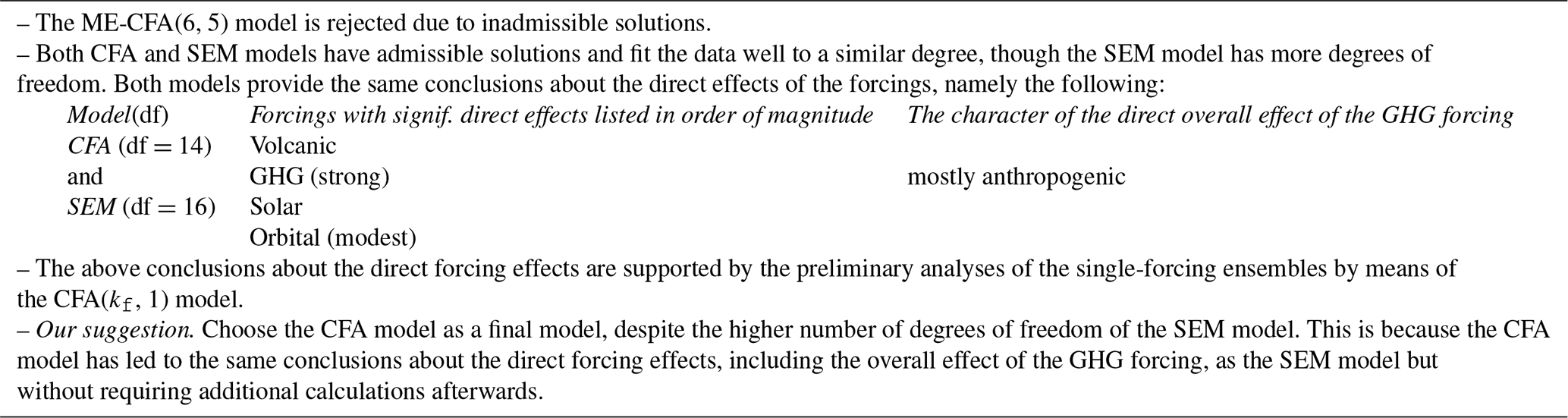
4.1.5 Summary of the analysis of the North America data

The ME-CFA(6, 5) model is rejected due to its under-identifiability, which caused either inadmissible solutions or inability of the estimation procedure to converge to a solution.

In contrast, both CFA and SEM models fit the data well and have admissible solutions. Moreover, they lead to similar conclusions about the direct effects of the forcings of interest. The sole difference is that the CFA model suggests that the significant overall effect of the GHG forcing is mostly due to (global-scaled) anthropogenic changes in GHG concentrations, while the SEM model highlights the dominant role of (global-scaled) natural changes. For the period of interest, both conclusions seem to be defensible and realistic from the climatological point of view.

Also, both CFA and SEM models demonstrated a stable performance and a very low sensitivity to starting values for the parameter estimates. However, the SEM model estimates two fewer parameters than the CFA model. So, in terms of the number of the parameters, the SEM model is simpler than the CFA model, though its underlying structure is more sophisticated from a climatological point of view. A lower number of parameters entails a higher number of degrees of freedom. More precisely, the SEM model has 2 more degrees of freedom, which increases the power of the χ² test statistic, whose values, in addition, turned out to be lower for the SEM model. For example, for data set no. 1, the model χ² test statistic was 15 and 9.5 for the CFA and SEM models, respectively. One can also see that the SRMR values are lower for the SEM model than for the CFA model (e.g. for data set no. 1, SRMR is 0.065 for the CFA model, while for the SEM model, SRMR equals 0.052). Taking into account the difference in the degrees of freedom, we may say that the SEM model fits the data substantially better than the CFA model.

All these points together speak in favour of the SEM model. Therefore, our suggestion is to choose the SEM model as an adequate approximation of the underlying latent structure of the simulated annual-mean temperature data for the region of North America during 850–1849 CE.

4.2 Overview of the results for the remaining regions

The brief summaries of the results for the remaining regions are presented in Tables 9–14.

Table 9 Summary of the result for Europe, summer (JJA) mean temperature, 850–1849 CE.

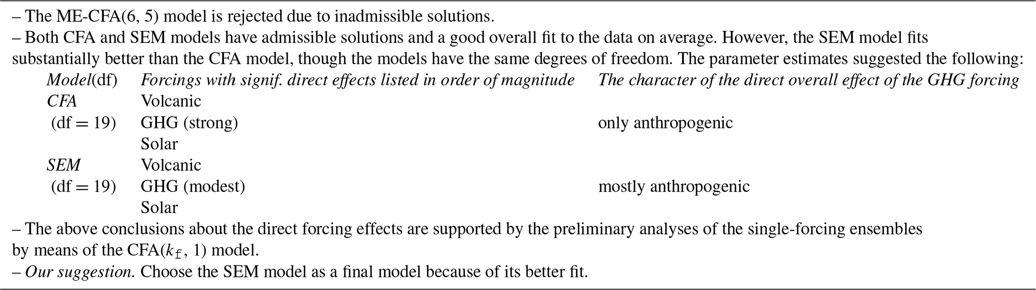
Table 10 Summary of the result for the Arctic, annual-mean temperature, 850–1849 CE.

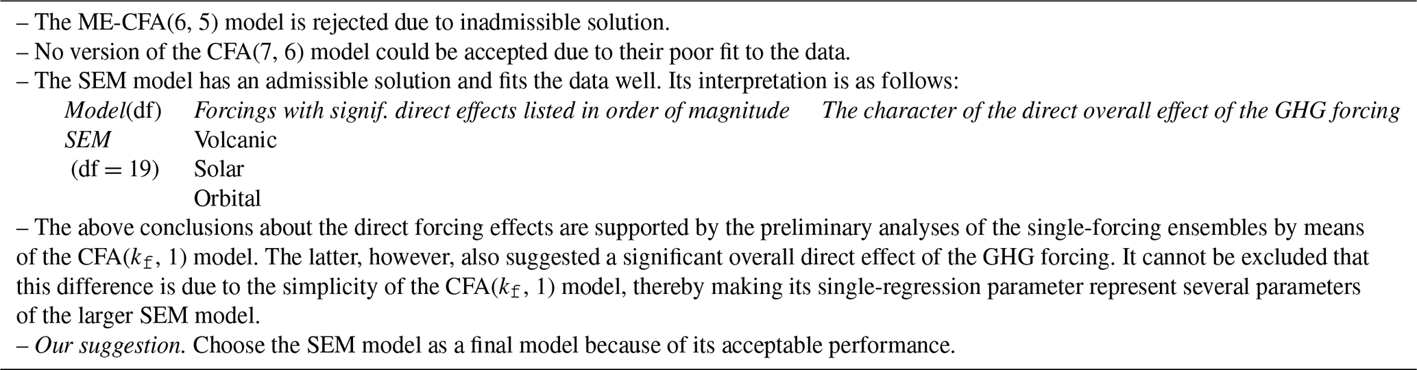
Table 11 Summary of the result for South America, summer (DJF) mean temperature, 850–1849 CE.

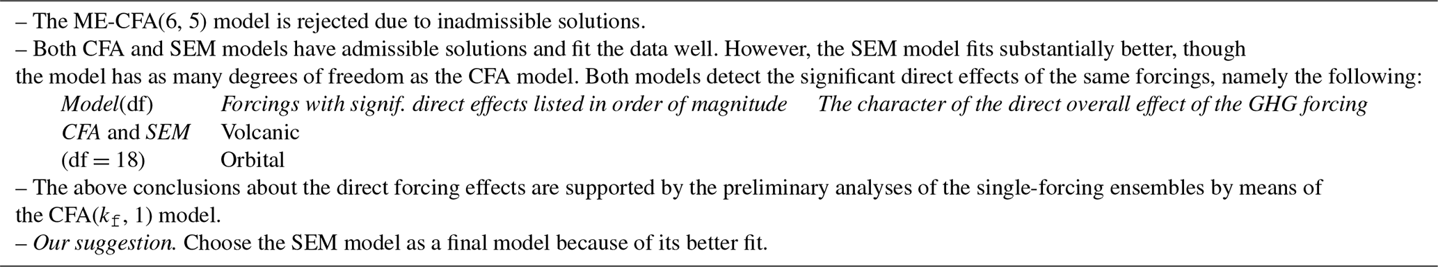
Table 12 Summary of the result for Antarctica, annual-mean temperature, 850–1849 CE.

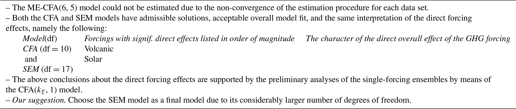
Table 13 Summary of the result for Asia, summer (JJA) mean temperature, 850–1849 CE.

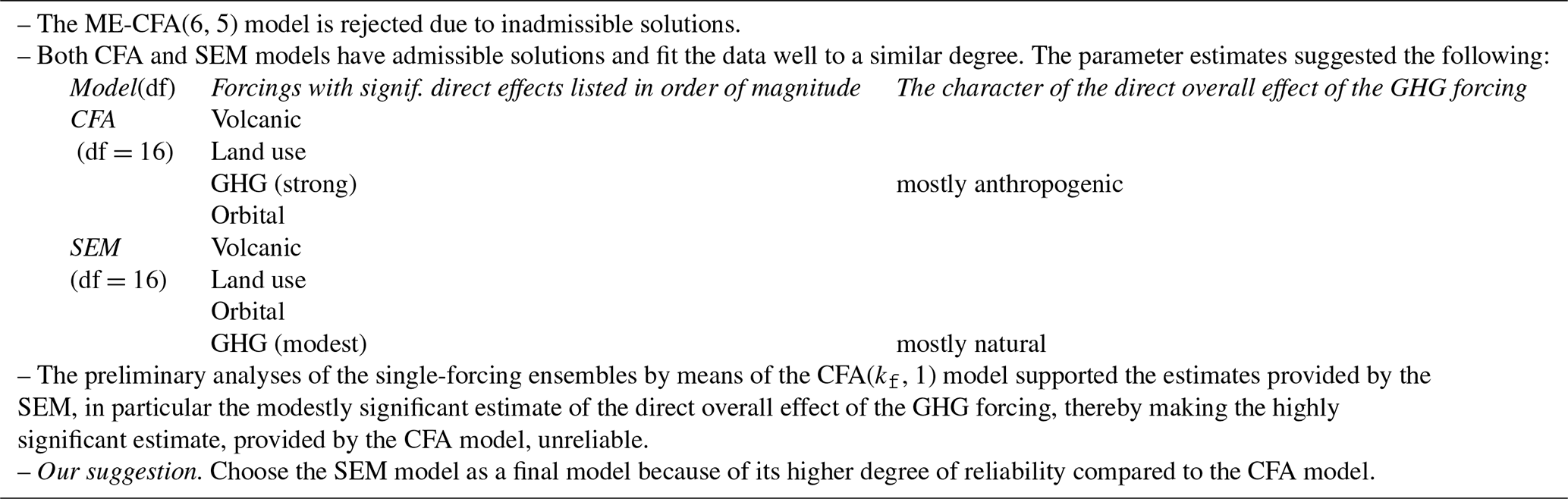
Table 14 Summary of the result for Australasia, warm-season (Sept–Feb) mean temperature, 850–1849 CE.

4.3 Discussion

According to the summaries provided, the SEM model has been chosen as a final model for all regions/seasons considered, except for Australasia. This result, first of all, indicates a complex causal structure of the simulated temperature data analysed, which required freeing up various causal links not permitted in the two other statistical models. For the region of Australasia, it was decided to choose the CFA model as a final model in accordance with the principle of parsimony.

All final models seem to have a climatologically defensible interpretation. Summarising the results per forcing, we may say the following:

• The direct effect of the volcanic forcing is well pronounced in all seven regions/seasons. In all cases, the volcanic forcing is found to have by far the strongest effect on the simulated temperatures, as compared to the effect from the other forcings.

• The direct effect of the orbital forcing is well detected in the simulated temperatures in three regions: the Arctic, Asia, and South America. A modest effect of the forcing is detected in the simulated Australasia warm-season mean temperatures. No effect of the orbital forcing is found in the simulated temperatures in North America, Europe, and Antarctica.

• A significant direct effect of the solar forcing is detected in five of the seven regions/seasons. No effect of the solar forcing is found in the simulated Asia (JJA) and South America (DJF) temperatures.

  Comment. We refrain from trying to explain this anomalous result for temperatures over these two regions, but we note that our result differs from results presented in a climate model simulation study made by Servonnat et al. (2010). They investigated the influence on temperatures of solar variability, carbon dioxide, and orbital forcing between 1000 and 1850 CE in the IPSLCM4 model. It can be seen in their Fig. 6c that solar variability has a significant influence (at the 0.05 level according to a Student's t test) on simulated (DJF) temperatures over much of a region that corresponds to the South America region used in our investigation. However, their simulations were driven with a solar irradiance forcing that has about 2.5 times higher amplitude, in terms of watts per square metre (W m⁻²), compared to the forcing used in the CESM simulations that we analyse. Thus, statistical significance of a solar forcing signal should be more easily reached in their study. We recognise this as an issue to be addressed in future studies that could hopefully provide better understanding of why the simulated effect of solar forcing on temperatures is significant in some regions but not in others. Indeed, the findings of Servonnat et al. (2010) indicate regional and seasonal differences in the effect from all three investigated forcings, where areas of significant versus insignificant temperature responses differ among the forcings.

• A significant overall direct effect of the GHG forcing is detected in four of the seven regions/seasons. Concerning the remaining three regions (Arctic, South America, and Antarctica), no effect of the GHG forcing is found in the corresponding simulated temperatures. In the regions where the effect of the GHG forcing was detected, its character was described by the final models as follows:

  • In the North America region, the SEM model suggests that the temperature response to the reconstructed GHG forcing is of a mixed character. That is, it represents the (annual) temperature response to both natural and anthropogenic changes, though the effect of natural changes is better seen than the effect of anthropogenic ones.

  • In the Europe region, the SEM model detects a stronger effect of anthropogenic changes (probably in the last about 1 century of data), while the effect of the natural changes was weakly pronounced.

  • In the Asia region, the SEM model suggests that the overall (summer) temperature response to the GHG forcing is of a mixed character with a dominating natural component. The anthropogenic component seems to be very weak.

  • In the Australasia region, the CFA model detects a dominating anthropogenic component in the strong overall (warm-season) temperature response to the GHG forcing. The natural component seems to be very weak. Importantly, even the SEM model led to the same conclusion.

• A significant direct effect of the land-use forcing is detected in only one of the seven regions/seasons, namely, in the Asia (JJA) mean temperatures.

• No effect of the interactions between the external forcings, leading to deviations from the additivity of the forcing effects, was found by the final statistical models in any of the seven regions/seasons.

Concerning the conclusions about the estimated forcing effects, it is essential to keep the following in mind:

• All of them are only justified for the particular climate model, period, regions, and seasons investigated in the analysis.

• The availability of simulated data was one of the important factors determining the complexity of the statistical models analysed. The absence of the climate model simulations, driven by various combinations of the five forcings of interest, led to a substantial simplification of the climatological relationships modelled in the statistical models presented. Nevertheless, the conclusions about the effect of the five forcings under consideration presented in the summaries are judged to be realistic and climatologically defensible.

5 Conclusions

The main aim of the present numerical experiment is to evaluate and compare the performance of three statistical models by fitting them to one and the same simulated temperature data set. The models are as follows:

1. the measurement error (ME) model, used in many D&A studies and there referred as to the method of “optimal fingerprinting” (here, rewritten as a factor model);

2. the confirmatory factor analysis (CFA) model;

3. the structural equation modelling (SEM) model.

Each statistical model provides estimates of direct effects of forcings on the temperature and contains the same latent variables representing unobservable temperature responses to forcings respective the internal processes. As a matter of fact, each model belongs to one and the same class of structural equation models with latent variables. Despite the similarities, the models have substantial differences. The following is a brief description of the main characteristics of the models relevant to our analysis:

1. The ME model estimates the forcing effects in accordance with the total least squares estimation approach under the condition that all latent temperature responses to the forcings in question are related to each other through correlation coefficients, regardless of the climate-relevant properties of the forcings. Within our study, this ME model is rewritten as a CFA model (hence the designation ME-CFA model), which facilitated the assessment of the overall model fit and the judgement of whether parameter estimates are admissible or not.

2. The CFA model, in contrast to the ME model above, allows for the modelling of mutually uncorrelated latent temperature responses to forcings but, just as the ME model above, does not allow for any causal relationships between them.

3. The SEM model is the most complex model, allowing for both uncorrelated latent temperature responses to forcings and various causal relationships between all model variables, including the latent ones.

The data, used in the analysis, consist of simulated temperatures obtained with the CESM Earth system model, covering the period of 850–1849 CE. The regions of interest coincide with the seven PAGES 2k regions: Europe, North America, Arctic, Asia, South America, Australasia, and Antarctica. Each statistical model above takes into account the fact that the CESM climate model was driven by five specific (reconstructed) forcings: the orbital, volcanic, and solar forcings, each of which is a purely natural forcing, the anthropogenic land-use forcing, and the GHG forcing, which may contain both natural and anthropogenic components.

A key feature of the present numerical experiment is that observational temperature data, or more precisely, the (real-world) observational data, are replaced by data from a climate model simulation forced by all five (reconstructed) forcings under study. This replacement makes it reasonable to accept the assumption that the simulated latent temperature responses to forcings, embedded in the simulated observable temperatures, are correctly represented regarding their magnitude and shape of their temporal evolution, compared to the corresponding latent temperature responses embedded in the pseudo-true temperature. Given this knowledge, a poor model fit to the data can be attributed to incorrectly specified unknown underlying relationships between the variables.

A good model fit, on the other hand, was only one of the three criteria for choosing a final model among the three statistical models studied. The two other criteria were as follows:

• The solution provided by the model is statistically admissible and climatologically defensible.

• The model demonstrates a stable performance across all data sets, including a different realisation of the pseudo-true temperature available for the region in question.

One of the important findings of our study is that the SEM model has been chosen as a final model for six of the seven regions/seasons considered. For the remaining region, the CFA model was chosen as a final model. Regarding the ME-CFA model, the experiment showed that this statistical model has to be rejected for all regions/seasons. This is because the estimation procedure of the ME-CFA model either failed to converge to a solution or resulted in inadmissible solutions.

One of the possible explanations of this result can be a complex causal structure of the data, not reflected in the ME-CFA model. Another possible explanation is that the estimation procedure of its parameters becomes unstable under the weak-signal regime observed for each regional data. However, the fact that this statistical model has been rejected in our analysis for all specific regional data does not imply that the model is inappropriate in other studies (either preceding or future ones). For another climate model, another set of forcings, and other regions and periods, ME-CFA models might turn out to be sufficient for describing the underlying latent structure of data.

A key idea of the numerical experiment presented (and of the framework on the whole) is that the researcher's thinking concerning the statistical modelling of climatological relationships should not be limited to a single statistical model. As underlined by the observed results, the availability of several statistical models is a basis for flexible evaluations of climate models concerning the representation of temperature responses to climate forcings. The degree of flexibility in choosing appropriate statistical models can further be increased by further modifications and improvements of our statistical models.

As a final comment, we would like to point out that the performance of the framework suggested was studied only for zero noise in the pseudo-observational data. However, as real observational data may contain significant and varying amounts of non-climatic noise, it is highly desirable to investigate its performance (in particular, the performance of the models chosen as final models) for more realistic levels of added noise, similar to what is found in real climate proxy data for past temperature variations. These investigations can also be complemented by the analysis of empirical coverage rates of approximate confidence intervals for parameter estimates that may differ from their nominal levels due to the approximative nature of the distributions of the parameter estimates, especially for endogenous parameters whose asymptotic variances are functions of several parameter estimates and are calculated using the delta method.