the Creative Commons Attribution 4.0 License.
the Creative Commons Attribution 4.0 License.
 | 16 May 2022
Comparing climate time series – Part 3: Discriminant analysis
Michael K. Tippett
In parts I and II of this paper series, rigorous tests for equality of stochastic processes were proposed. These tests provide objective criteria for deciding whether two processes differ, but they provide no information about the nature of those differences. This paper develops a systematic and optimal approach to diagnosing differences between multivariate stochastic processes. Like the tests, the diagnostics are framed in terms of vector autoregressive (VAR) models, which can be viewed as a dynamical system forced by random noise. The tests depend on two statistics, one that measures dissimilarity in dynamical operators and another that measures dissimilarity in noise covariances. Under suitable assumptions, these statistics are independent and can be tested separately for significance. If a term is significant, then the linear combination of variables that maximizes that term is obtained. The resulting indices contain all relevant information about differences between data sets. These techniques are applied to diagnose how the variability of annual-mean North Atlantic sea surface temperature differs between climate models and observations. For most models, differences in both noise processes and dynamics are important. Over 40 % of the differences in noise statistics can be explained by one or two discriminant components, though these components can be model dependent. Maximizing dissimilarity in dynamical operators identifies situations in which some climate models predict large-scale anomalies with the wrong sign.


Comparing time series is a common task in climate studies, yet there are few rigorous criteria for deciding whether two time series come from the same stationary process. Such comparisons are vital in climate studies, particularly for deciding whether climate models produce realistic simulations. Part I of this study (DelSole and Tippett, 2020) derived a test for the hypothesis that two univariate time series come from the same stationary autoregressive process. Part II generalized this test to multivariate time series (DelSole and Tippett, 2021a). However, the decision that two processes differ provides no information about the nature of those differences. The purpose of this paper is to develop optimal diagnostics of differences between multivariate stochastic processes. Such diagnostics may help to identify errors in climate models and suggest ways to correct them.
The starting point of our approach is the objective criterion derived in Part II for deciding whether two multivariate time series come from the same process. This criterion assumes that each multivariate time series comes from a vector autoregressive (VAR) model. Part II derived the likelihood ratio test for equality of VAR parameters. The associated test statistic, called a deviance statistic, depends on all parameters in the VAR models, as it should, but in specific applications it may be dominated by particular aspects of the VAR models, such as differences in noise processes or differences in dynamics. In this paper, we first show that the deviance can be partitioned into two terms such that one term measures differences in noise processes and the other term measures differences in dynamics. Under suitable assumptions, these terms are independent. Then, the individual terms are further decomposed using discriminant analysis techniques. Discriminant analysis finds linear combinations of variables that maximize some quantity.
When applied to diagnose dissimilarity in noise processes, discriminant analysis yields a procedure that is similar to principal component analysis and other related techniques for diagnosing variability (Schneider and Griffies, 1999; DelSole et al., 2011; Wills et al., 2018). When applied to diagnose dissimilarity in dynamics, discriminant analysis yields a procedure that is equivalent to generalized singular value decomposition. Although both procedures have appeared in previous studies, no rigorous significance test accompanied these applications. In this work, these procedures emerge naturally from a rigorous statistical framework, and, as a result, they each have a well-defined significance test. A significance test is possible because each dissimilarity measure is based on prewhitened variables rather than on the original, serially correlated variables.
These new analysis techniques are applied to diagnose how variability of annual-mean North Atlantic sea surface temperature (SST) differs between observations and model simulations. It is found that differences in noise processes and differences in dynamics both play a significant role in explaining the overall differences. The components that dominate these differences are illustrated for a few cases. This paper closes with a summary and discussion.
This section briefly reviews the procedure derived in Part II for deciding whether two time series come from the same stochastic process. This procedure considers only stationary, Gaussian processes. Such processes are described completely by a mean vector and time-lagged covariance matrices. Standard tests for differences in these quantities (see chapter 10 of Anderson, 1984) assume independent data and therefore are not suitable for comparing serially correlated multivariate time series. Our approach is to fit a VAR model to data and then test equality of model parameters. Accordingly, consider a J-dimensional random vector zt, where t is a time index. A VAR model for zt is
where are constant J×J matrices, μ is a constant vector that controls the mean of zt, and ϵt is a Gaussian white noise process with covariance Γ. We refer to ϵt as the noise and as the AR parameters. The term model parameters refers to the set , which involves a total of independent parameters.
Typically, AR parameters characterize dynamics. For instance, some stochastic models are derived by linearizing the equations of motion about a time mean flow and parameterizing the eddy–eddy nonlinear interactions by a stochastic forcing and linear damping (Farrell and Ioannou, 1995; DelSole, 2004). Similar stochastic models can be derived by linear inverse methods (Penland, 1989; Winkler et al., 2001). Majda et al. (2006) showed that such stochastic models can be derived under suitable assumptions of a timescale separation (see the review by Gottwald et al., 2017). Realizations from these stochastic models, sampled at discrete time intervals, are indistinguishable from realizations of VAR models. In each of these models, the AR parameters characterize physical processes such as advection, dissipation, and wave propagation. Accordingly, we say that AR parameters characterize the dynamics of the system and that differences in AR parameters indicate differences in dynamics.
The model parameters can be estimated by the method of least squares, and the distributions of the estimates are asymptotically normal (Lütkepohl, 2005, Sect. 3.2.2). Accordingly, it proves convenient to express the VAR model as a regression model. Suppose Eq. (1) is used to generate N+p realizations . Then, these realizations can be modeled by
where 1 is an N-dimensional vector of ones, superscript T denotes the transpose operation, the rows of E are independent realizations of ϵt, and
Inferences based on the above regression model are identical to inferences based on the model , where in the latter model μ is omitted and X and Y contain centered variables in which the mean of each column is subtracted from that column. To simplify the analysis, we hereafter consider regression models of the form comprising centered variables. To account for centering, 1 degree of freedom per dimension should be removed at the appropriate steps below, but for brevity they will not be discussed further. With this understanding, we hereafter express our two VAR models in the form
where
M=Jp, and E1 and E2 are independent and distributed as
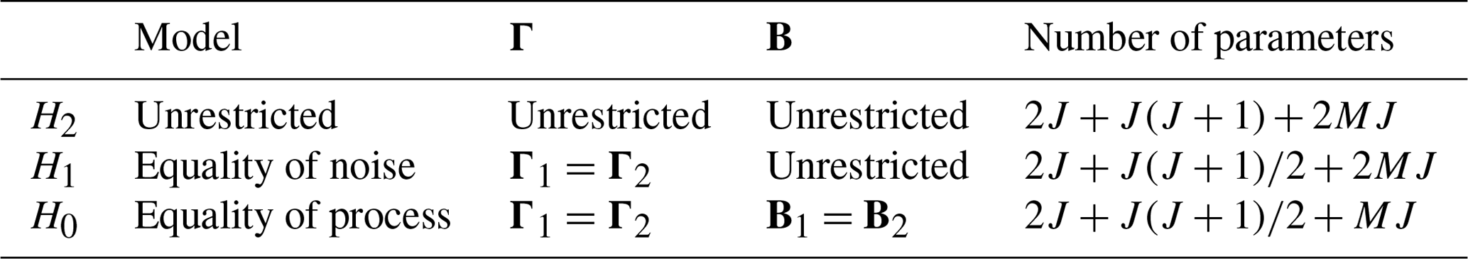
The null hypothesis is
Let B0 and Γ0 denote the common regression parameters and noise covariance matrix under H0, respectively. The total number of parameters estimated under H0 is , derived by summing 2J for μ1 and μ2, MJ for B0, and for Γ0. On the other hand, the case of unconstrained VAR processes is denoted as
The total number of parameters estimated under H2 is .
As discussed in Part II of this paper series, the bias-corrected likelihood ratio for testing H0 versus H2 is
where denotes the determinant and
and we have used the following operator for any matrix Z:
In our applications, and are positive definite, and this will be assumed hereafter.
MLEs and unbiased estimates are asymptotically equivalent. Hence, asymptotic theory (Hogg et al., 2019) gives the distribution of the deviance statistic under H0 as
If no difference in VAR models is detected, then the data are assumed to come from the same stochastic process.
Note that covariance matrices Γ1 and Γ2 characterize the residuals of the VAR models. If , then the process is white noise, and the above test reduces to the standard likelihood ratio test for differences in covariance matrices (e.g., see Anderson, 1984). If the process is VAR(p), then Yi−XiBi transforms the correlated process Yt into an uncorrelated white noise process. Such a transformation is called a prewhitening transformation (Box et al., 2008). In practice, Bi is not known, and hence the sample estimate is substituted, yielding an approximately white noise process. Accordingly, is the covariance matrix of the prewhitened variables and characterizes the noise statistics.
If H0 is rejected, then a difference in VAR models is said to be detected. However, this result does not tell us the nature of those differences. A natural question is whether the difference can be attributed to a difference in noise statistics or a difference in AR parameters. To answer these questions, we consider a hypothesis that is intermediate between H0 and H2, namely,
As a shorthand, H1 will be called equality of noise. Under H1, the maximum likelihood estimates of B1 and B2 are Eqs. (6) and (7), and the (bias-corrected) maximum likelihood estimate of the covariance matrix Γ is
It follows that the deviance statistic for testing H0 versus H1 is
and the deviance statistic for testing H1 versus H2 is
It is readily verified that the sum of these deviances gives the original deviance:
In the next section, we will see that D1:2 measures differences in noise covariances, and D0:1 measures differences in AR parameters. Under this interpretation, Eq. (16) decomposes total deviance into a part due to differences in noise statistics and a part due to differences in AR parameters.
Table 1Table summarizing the hypotheses considered in the hierarchical test procedure.
Testing significance requires knowing the sampling distributions of D0:1 and D1:2. Under H1, standard regression theory indicates that and each have independent Wishart distributions (Fujikoshi et al., 2010, Theorem 7.2.1). Importantly, these distributions are independent of the model parameters. Since D1:2 depends only on and , it too has a distribution that is independent of the model parameters (under H1). For large sample sizes, this distribution approaches a chi-squared distribution with degrees of freedom (see Hogg et al., 2019, Theorem 6.5.1), which we denote as
In contrast, the distribution of D0:1 is more complicated. In the special case in which H1 is true, the hypothesis of equal AR parameters can be tested as a standard problem in general linear hypothesis, which yields a statistic that depends only on and . Again, the sampling distribution is independent of the model parameters. Since D0:1 depends only on and , we may infer that the distribution of D0:1 is also independent of the model parameters. In this case, asymptotic theory indicates that, for large sample sizes, the distribution is
As expected, for consistency, the sum of the degrees of freedom in Eqs. (17) and (18) equals that in Eq. (12).
However, if H1 is not true (i.e., the noise covariances differ), then the distribution of D0:1 depends on how the noise covariances differ. A similar situation arises with the t-test. Recall that the t-test assesses equality of means assuming equal variances. However, if the variances are unequal, the t-test is inappropriate because the distribution of the t-statistic depends on the ratio of variances. This is the central issue in the Behrens–Fisher problem, for which there are multiple tests with various probabilistic interpretations (Scheffé, 1970; Kim and Cohen, 1998). Our procedure would reduce to the t-test if the hypothesis μ1=μ2 were tested in the case of J=1 and vanishing AR parameters. Since the intercept μ is merely a special case of a regression matrix B, one can anticipate that testing equality of regression parameters would also lead to a sampling distribution that depends on the difference in noise covariances. Therefore, testing equality of AR parameters without assuming equality of noise covariances would lead to complications analogous to those associated with the Behrens–Fisher problem. To avoid these complications, we test equality of AR parameters under the assumption of equal noise covariances. This restriction is of the same kind as that invoked routinely in the t-test.
Given the above restriction, the hypotheses in our problem are summarized in Table 1 and nested as . A natural procedure is to first test equality of noise covariances and then, if that hypothesis is accepted, test equality of regression parameters under the restriction of equal noise covariances. This stepwise testing procedure is a special case of a general procedure discussed by Hogg (1961). Specifically, Hogg (1961) showed that if the maximum likelihood estimates of a set of nested hypotheses are completely sufficient statistics, then the resulting test statistics are stochastically independent, and the most restrictive hypothesis can be tested by testing a sequence of intermediate hypotheses. Hogg's procedure leads to the following stepwise procedure. First, D1:2 is tested for significance based on Eq. (17). If it is significantly large, then we decide that the noise covariances differ and stop testing. If D1:2 is not significant, then D0:1 is tested for significance based on Eq. (18). If it is significant, then we decide that the noise covariances are equal, but the AR parameters differ. If D0:1 is not significant, then we conclude that no significant difference in VAR models is detected. This procedure involves two steps performed at the α100 % level. Because the tests are stochastically independent, the family-wise error rate (FWER) for testing H0 is
Thus, if each step is performed at the α=5 % level, then the corresponding FWER is 9.75 %.
If D1:2 is significantly large, then the noise covariances are said to differ. However, this conclusion does not tell us the nature of those differences. The question arises as to how to describe the difference between two covariance matrices in an efficient manner. Flury (1986) suggested using the linear combination of variables with extreme ratios. This approach is a generalization of principal component analysis (PCA), but instead of maximizing variance itself, a ratio of variances is optimized. We call this approach covariance discriminant analysis (CDA). A review of CDA is given in DelSole and Tippett (2022). CDA is a generalization of the discriminant analysis used in classification studies. We refer to both methods as discriminant analysis.
Discriminant analysis begins by considering the linear combination of prewhitened variables,
where qY is a vector containing the coefficients of the linear combination. The resulting vector r(k) is a time series called a variate. The corresponding sample variances are
and the corresponding deviance statistic D1:2 for the scalar variables r(1) and r(2) is
where Eq. (13) is used to define
Substituting Eq. (21) into Eq. (20) and using elementary properties of the log function yields
where θ is the ratio of noise variances given by the Rayleigh quotient
The stationary values of d1:2 are found by using the chain rule:
The function d1:2(θ) is U-shaped with a minimum at θ=1, but the stationary value at θ=1 is not of interest since it is a minimum. For θ>1 the only stationary values occur at , and for θ<1 the only stationary values occur at . Both cases lead to the same condition , which in turn leads to the generalized eigenvalue problem
(see Seber, 2008, result 6.59). This eigenvalue problem has at most J distinct solutions. Because d1:2(θ) is a U-shaped function, large deviances arise from large and small values of θ. This is sensible because deviance is a measure of the difference in variance, and two variances may differ because one is much greater or much less than the other. We order the eigenvalues by their value of d1:2(θi), which means that the eigenvalues generally are not ordered from largest to smallest; for instance, the leading component might have the smallest eigenvalue. Let the corresponding eigenvectors be . Then, the maximum possible deviance is obtained from qY,1, which yields time series Eq. (19) and has deviance D1:2(θ1).
When examining the leading eigenvalue θ1, it is informative to compare to a significance threshold under H1. This threshold can be estimated by Monte Carlo methods. Specifically, one generates samples from Eqs. (2) and (3) using . The sampling distribution is independent of B1 and B2, and hence they can be set to zero in the Monte Carlo model. From these samples, one computes the noise covariance matrices, solves the generalized eigenvalue problem Eq. (23), and then repeats this procedure numerous times to build an empirical distribution of θ1. The resulting test is equivalent to the union-intersection test (Mardia et al., 1979). We emphasize that this test is done only as a reference for judging the significance of a single eigenvalue and is not meant to replace the above test based on D1:2, which depends on all the eigenvalues.
It can be shown that the variates corresponding to the eigenvectors are uncorrelated (see Appendix A). Recall that eigenvectors are unique up to a multiplicative constant. It is conventional to normalize the eigenvectors of Eq. (23) so that the denominator in Eq. (22) is one, or equivalently, that the variates each have unit variance. Under this normalization, the prewhitened variables may be decomposed as
where is a loading vector defined as
We call the individual term a noise discriminant. Equation (24) shows that prewhitened variables can be decomposed into a sum of independent noise discriminants, where is a time series describing the temporal structure of the noise discriminant, and is a loading vector describing the spatial structure of the noise discriminant. Appendix A also shows that
That is, D1:2 is the sum of deviances of the individual noise discriminants. Thus, the decomposition simultaneously decomposes the prewhitened variables and the deviance D1:2 into a sum of independent components. If a few noise discriminants dominate the total deviance (either because the associated θj is much greater than or much less than one), then those discriminants provide a low-dimensional description of differences in noise variances.
If D1:2 is sufficiently small, then no difference in noise processes is detected and we turn to D0:1. If D0:1 is significantly large, then we conclude there is a difference in dynamics, but the nature of those differences is unknown. Again, we seek linear combinations that maximize D0:1, consistent with discriminant analysis. Under H0, the prewhitening transformation depends on rather than and , and therefore we introduce the prewhitened variables under H0,
We continue to use to denote a projection vector, loading vector, and variate, respectively, but the interpretation differs from that in Sect. 4 because here we are maximizing D0:1 rather than D1:2. A linear combination of is
which has variance
The corresponding deviance statistic from Eq. (14) is then
where
Because d0:1(λ) is a monotone function of λ, maximizing d0:1(λ) is equivalent to maximizing λ, which leads to the eigenvalue problem
Let the eigenvalues be ordered from largest to smallest, i.e., , and let the corresponding eigenvectors be denoted as . The rest of the procedure is similar to that in Sect. 4, and for brevity we simply state the final results. Specifically, the variates are uncorrelated, and the loading vectors are
and if the eigenvectors are normalized as , then the prewhitened variables are decomposed as
and the deviance is decomposed as
We call a difference-in-dynamics component. Identity Eq. (30) shows that D0:1 can be decomposed as a sum of deviances of the individual components. The significance threshold of λ1 under H0 can be estimated by the same Monte Carlo method discussed in Sect. 4, except that Eq. (28) is solved instead of Eq. (23).
Although we have decomposed and D0:1, it is not obvious how this elucidates differences in dynamics. After all, dynamics are contained in and , but these quantities do not appear explicitly in the above decomposition. In Appendix C, we show that the loading vectors appear in the generalized singular value decomposition (GSVD) of B1−B2,
where are singular values, are left singular vectors, and are right singular vectors. In contrast to the standard SVD, the left and right singular vectors satisfy the generalized orthogonality conditions
This decomposition is equivalent to an SVD of a suitably transformed B1−B2 (Appendix C; see also Abdi and Williams, 2010). The matrix ΣH is a covariance matrix defined in Appendix B (see B3). Note that if ΣH=I and , then Eq. (32) would be Euclidean norms and Eq. (31) would be the standard SVD. We call si a difference-in-dynamics singular value. Appendix C further shows that D0:1 can be decomposed as
si can be interpreted as measuring the magnitude of the difference in dynamics, and describes the manifestation of these differences in the prewhitened variables. Furthermore, Eq. (33) shows that the deviance D0:1 can be decomposed as a sum of the deviances of the individual components. Although a standard SVD would also decompose , it would not simultaneously decompose D0:1 into a sum of terms, each of which depends only on a single component. If the sum in Eq. (33) is dominated by the first few components, then differences in AR parameters can be described by those components. We call this decomposition a difference-in-dynamics SVD.
To further clarify the decomposition Eq. (31), note that the form of Eqs. (2) and (3) implies that qX,j projects X onto the jth difference-in-dynamics component. The corresponding loading vector is
It follows from this and the first orthogonality constraint in Eq. (32) that the loading vectors and projection vectors qX,j form a bi-orthogonal set satisfying . Therefore, multiplying the transpose of Eq. (31) by yields
This equation indicates that defines an initial condition, while the vector describes the corresponding difference in response, and si measures the amplitude of the difference in response. In Appendix C, we show that
where is a distance measure defined as
for any vector a and positive definite matrix A. Thus, given the initial condition , the squared singular value is the ratio of the dissimilarity in response over the initial amplitude. The dissimilarity in response is measured with respect to a norm based on the average noise covariance matrix . Thus, the numerator in Eq. (35) is a signal-to-noise ratio, which is an attractive basis for measuring differences in responses. Because satisfies the same optimization properties as λj, it follows that maximizes Eq. (35), or equivalently, it maximizes the dissimilarity in response subject to (Noble and Daniel, 1988, Theorem 10.22). The latter condition defines a surface of constant probability density under 𝒩(0,ΣH). Thus, produces the biggest difference in response among all “equally likely” vectors under 𝒩(0,ΣH).
SVD has been used in past studies of empirical dynamical models (e.g., Penland and Sardeshmukh, 1995; Winkler et al., 2001; Shin and Newman, 2021), so it is of interest to discuss how the GSVD differs from past applications. For p=1, the VAR model with time step τ is mathematically equivalent to a linear inverse model (LIM) integrated to time τ. In LIM studies, the SVD is used to identify the “optimal initial condition” and the “maximum amplification curve”, which are derived by applying a standard SVD directly to the propagator . Thus, one obvious difference is that the SVD in this paper diagnoses differences in dynamics rather than dynamics itself. A more fundamental difference is that the standard SVD uses the Euclidean norm to constrain the initial and final vectors, which yields singular values that depend on the coordinate system. In contrast, difference-in-dynamics singular values are invariant to invertible linear transformations of Y and therefore are independent of the coordinate system (this is proven in Appendix D).
We now apply the above procedure to diagnose dissimilarities in internal variability of annual mean North Atlantic SST (NASST; N) between observations and climate models. Our choices for climate models, observations, and VAR model were discussed in Part II. We first summarize these relevant results from Part II.
6.1 Summary of NASST analysis in Part II
In Part II, we applied the difference-in-VAR test to pre-industrial control runs from phase 5 of the Coupled Model Intercomparison Project (CMIP5 Taylor et al., 2012). These simulations contain only internal variability and do not contain forced variability on interannual timescales. We analyzed 36 control simulations of length 165 years.
For dimension reduction, NASST fields were projected onto the leading Laplacian eigenvectors in the Atlantic basin. The number of Laplacian eigenvectors J and the order of the VAR model p were chosen using an objective criterion called the Mutual Information Criterion (MIC; DelSole and Tippett, 2021b). This criterion is a generalization of Akaike's information criterion to random predictors and selection of predictands. As discussed in Part II, this criterion selected different values of p and J for different CMIP5 models. To quantify differences using our difference-in-VAR test, a common VAR model must be selected. Which model should be selected? Choosing p too small may result in residuals that contain serial correlations, contradicting our distributional assumptions. Choosing p too large may result in overfitting. Of the two problems, overfitting is less serious because it is taken into account in the statistical test. The main negative impact of overfitting is the loss of statistical power. In this study, loss of power is not a concern because differences grow rapidly with p and J. For this reason, we advocate selecting the maximum p and J among the models selected by MIC. As documented in Part II, these considerations lead to selecting J=7 Laplacian eigenvectors and order p=1.
To assess model adequacy, we performed the multivariate Ljung–Box test (Lütkepohl, 2005, Sect. 4.4.3). After a Bonferroni correction, only 1 of the 36 CMIP5 models had detectable serial correlations, consistent with the expected rate, suggesting that VAR(1) with J=7 was adequate for our data. Our choice of p=1 leads to a model that is indistinguishable from an LIM sampled at discrete time steps. Numerous studies have shown that LIMs provide reasonable models of monthly-mean and annual-mean SSTs (Alexander et al., 2008; Vimont, 2012; Zanna, 2012; Newman, 2013; Huddart et al., 2016; Dias et al., 2018) and can predict tropical SSTs with a skill close to that of state-of-the-art coupled atmosphere–ocean models (Newman and Sardeshmukh, 2017).
For observations, we used version 5 of the extended reconstructed SST data set (ERSSTv5; Huang et al., 2017) and considered the 165-year period 1854–2018. To remove forced variability, we regressed out either a second- or ninth-order polynomial function of time. For the sake of simplicity, we focus only on residuals from a quadratic. The CMIP5 and observation time series were split in half (82 and 83 years), and time series from the earlier half were compared to those in the latter half. The motivation behind this analysis was that if a time series comes from the same source, then the null hypothesis is true and the method should detect a difference at a rate consistent with the significance threshold, which was borne out by the results. Virtually all CMIP5 models were found to be inconsistent with observations. However, the nature of these differences was not diagnosed. The goal of this section is to diagnose these differences.
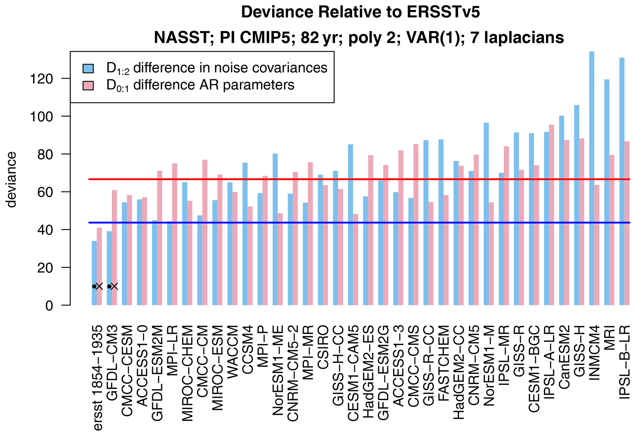
Figure 1The deviance statistics D1:2 (blue) and D0:1 (red) for comparing ERSSTv5 1854–1935 to 82-year segments from 36 CMIP5 pre-industrial control simulations and to ERSSTv5 1936–2018. The 5 % critical values for D1:2 and D0:1 are indicated by the horizontal blue and red lines, respectively. The dots indicate H1 is not rejected; i.e., equality of noise covariance matrices is not rejected.
6.2 Testing equality of noise covariances
First, we decompose the deviance as . The individual terms D0:1 and D1:2 are shown in Fig. 1. We test each term at the 5 % significance level. The corresponding critical values are indicated as horizontal lines in Fig. 1. In most cases, differences in both noise covariances and AR parameters contribute substantially to the total deviance. We reject H1 (i.e., equality of noise covariances) when D1:2 exceeds its critical value (i.e., when blue bars cross the blue line). The figure shows that D1:2 is significant for all but one model (GFDL-CM3), indicating that for most models the noise covariances differ between observations and CMIP5 models.
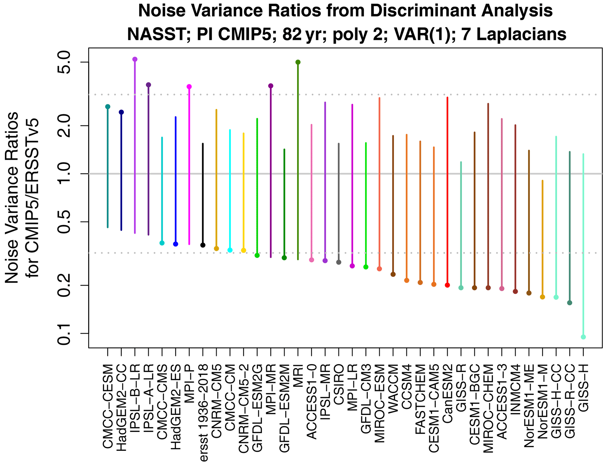
Figure 2Range of noise variance ratios for maximizing the noise deviance D1:2 between ERSSTv5 1854–1935 and 82-year segments from 36 CMIP5 pre-industrial control simulations. The horizontal dotted lines show the 2.5 % and 97.5 % significance thresholds under hypothesis H1. The dots identify the noise variance ratio that dominates the deviance (deviance measures the difference from one but does not distinguish between values greater than or less than one).
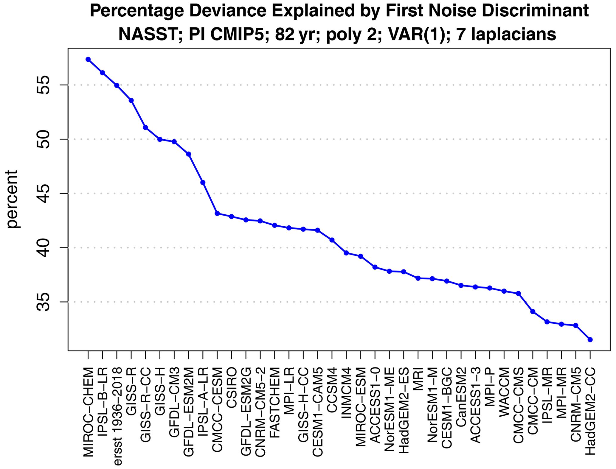
Figure 3Percent of deviance D1:2 explained by the first noise discriminant, for the variance ratios shown in Fig. 2.
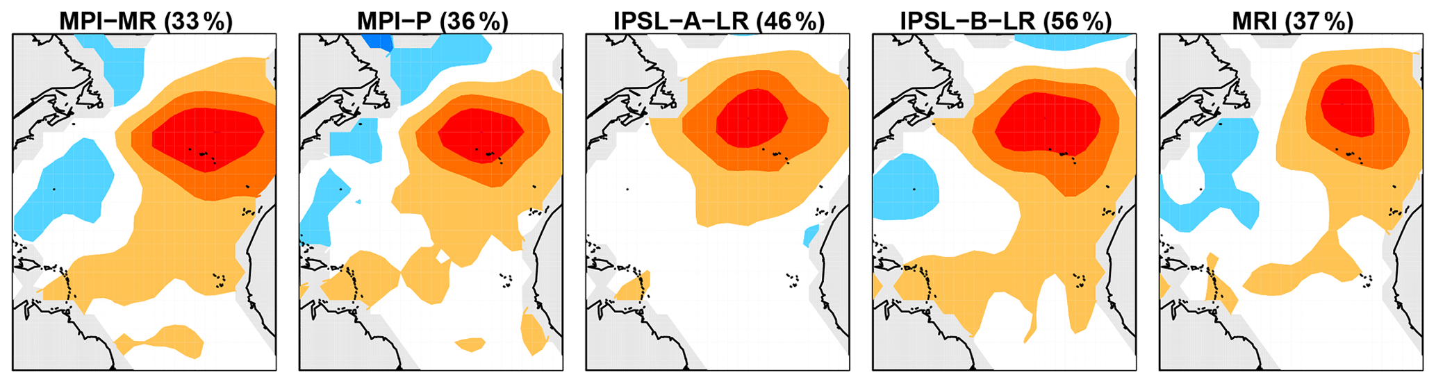
Figure 4Regression patterns between local SST and the discriminant associated with the largest model-to-observation variance ratio. Only regression patterns associated with significant maximum variance ratios are shown. Each regression pattern is scaled to have a maximum absolute coefficient of one and is then plotted using the same color scale (red and blue are opposite signs). The CMIP5 model and percent of deviance D1:2 explained by the discriminant are indicated in the title of each panel.
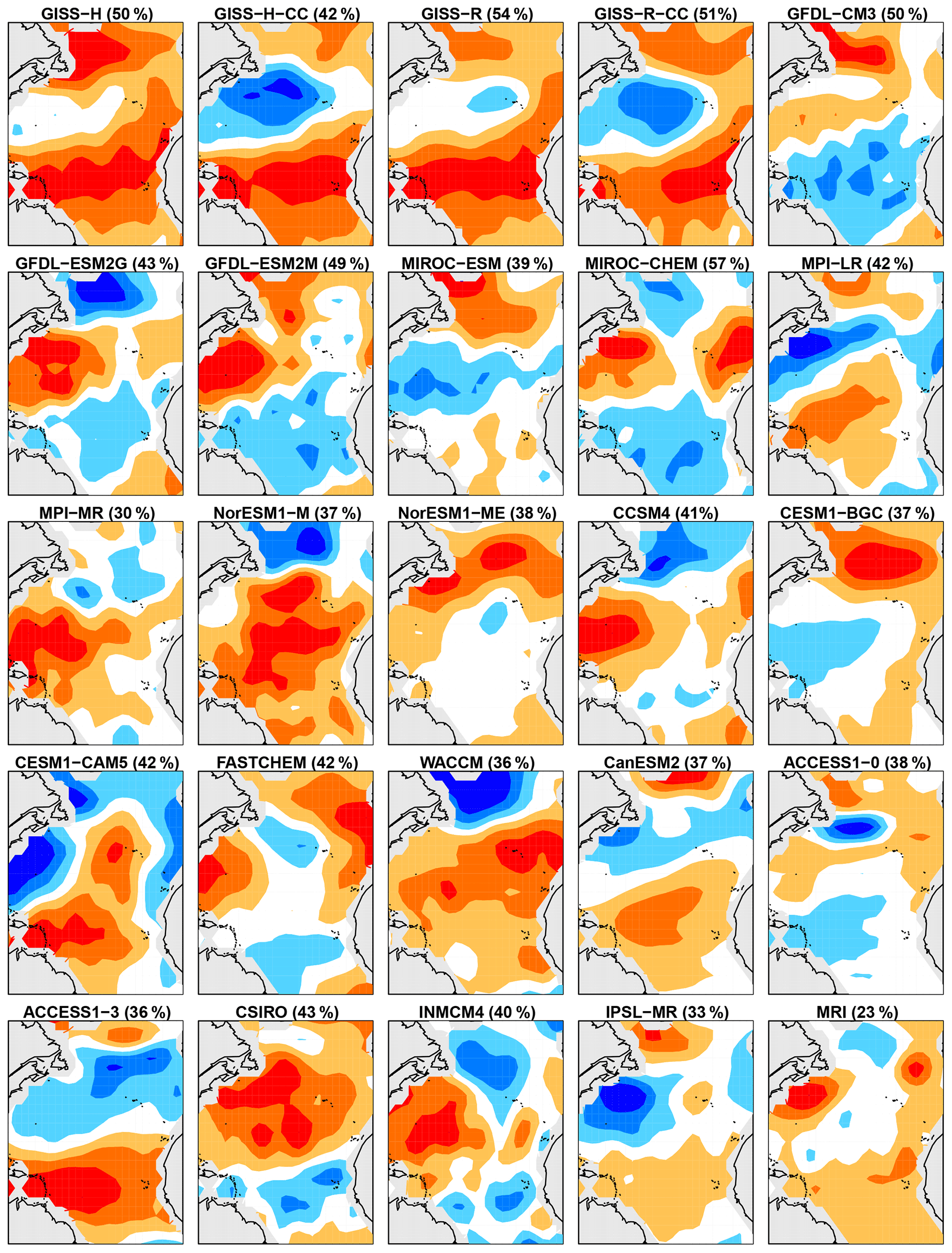
Figure 5Same as Fig. 4 except for discriminants associated with the smallest model-to-observation variance ratio (i.e., CMIP5 models whose stochastic noises are smaller than those in observations).
6.3 Diagnosing differences in noise covariances
To diagnose differences in noise covariances, we perform the discriminant analysis described in Sect. 4 to find the components that maximize D1:2. Specifically, observations in the first period are compared to models and observations in the second period. The corresponding ratios of noise variances θ are shown in Fig. 2. The ratio is defined as model over observations, so a ratio exceeding one indicates that the discriminant has a larger variance in the model than in observations. The horizontal dotted lines show the 2.5 % and 97.5 % significance thresholds for extreme ratios. The results show that most CMIP5 models have too little variance in their leading discriminant (where “leading” means the maximum value of θ1 or ).
It is worth mentioning that a significant extreme ratio is not always expected when a significant deviance is detected. Discriminant analysis is designed to compress as much deviance as possible into the fewest number of components. The extent of compression depends on the data. If little compression is possible (e.g., the deviances are spread uniformly in phase space), then the most extreme ratio may not be significant, but nevertheless the overall deviance may be significant because individual deviances accumulate. The fact that in some CMIP5 models the most extreme noise variance ratio is insignificant, despite the noise deviance being significant, simply means that the deviance cannot be compressed significantly into a single component.
The percent of deviance D1:2 explained by the leading discriminant is shown in Fig. 3. The leading discriminant explains more than 40 % of the deviance in about a half of the models. In these cases, the leading discriminant can provide an efficient basis for describing differences in noise covariances. Recall that these discriminants pertain to prewhitened variables. The time-lagged autocorrelation function of discriminant time series reveals little serial correlation (not shown).
To diagnose the spatial structure, we derive regression coefficients in which the observed local SST is the independent variable and in Eq. (19) is the dependent variable. Since the discriminants differ from model to model, differences in amplitude have complex interpretations, and hence for simplicity each regression pattern is scaled to have a maximum absolute coefficient of one. Figure 4 shows regression patterns for the case in which prewhitened variables in CMIP5 models have too much variance compared to ERSSTv5. As can be seen, the spatial structure of these discriminants is similar across CMIP5 models, suggesting a common model deficiency. The regression patterns associated with discriminants with too little (prewhitened) variance are shown in Fig. 5. Here, there is no obvious common structure across different models, although some patterns tend to be similar for CMIP5 models from the same institution.
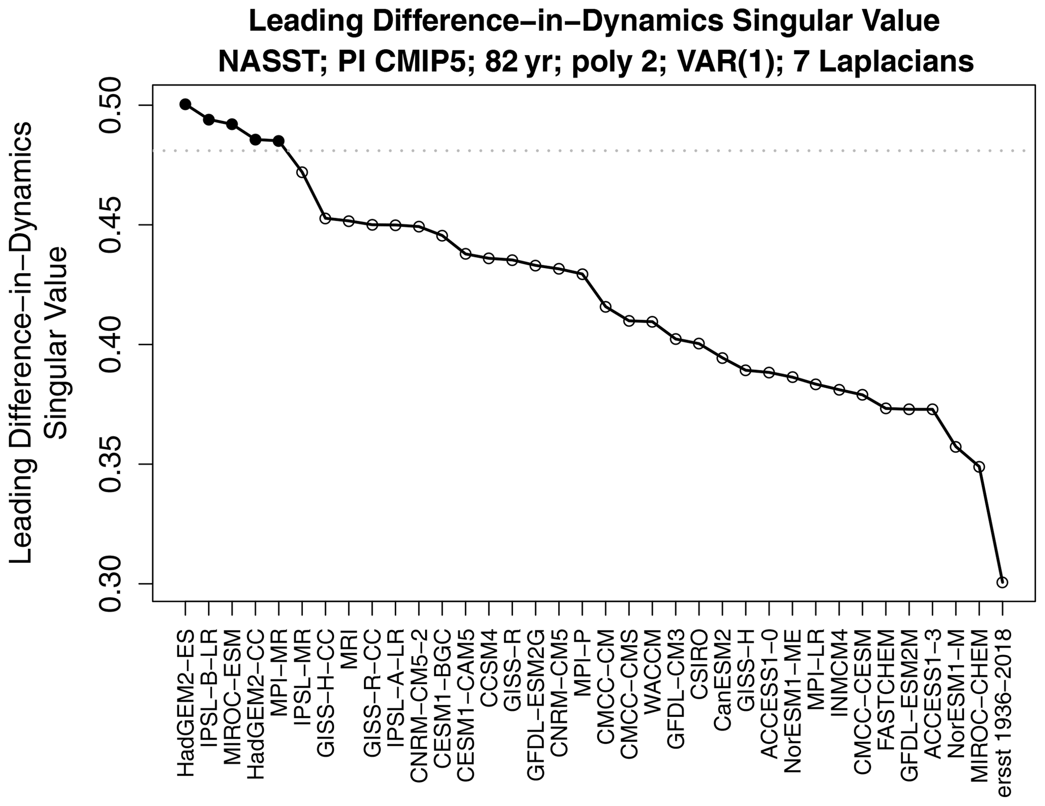
Figure 6The leading difference-in-dynamics singular value for each CMIP5 model. The 5 % significance threshold under H1 is shown as the dotted horizontal line. Significant and insignificant singular values under H1 are indicated by filled and open circles, respectively.
6.4 Diagnosing differences in dynamics
We now turn to diagnosing differences in AR parameters. Equality of AR parameters is rejected when D0:1 exceeds its critical value (i.e., when the red bars cross the red line), provided H1 is not rejected. However, H1 is rejected for virtually all models, so for these models, strictly speaking, the testing procedure halts before testing equality of AR parameters. Having noted this fact, we nevertheless proceed with discriminant analysis of D0:1 for the purpose of illustrating the procedure.
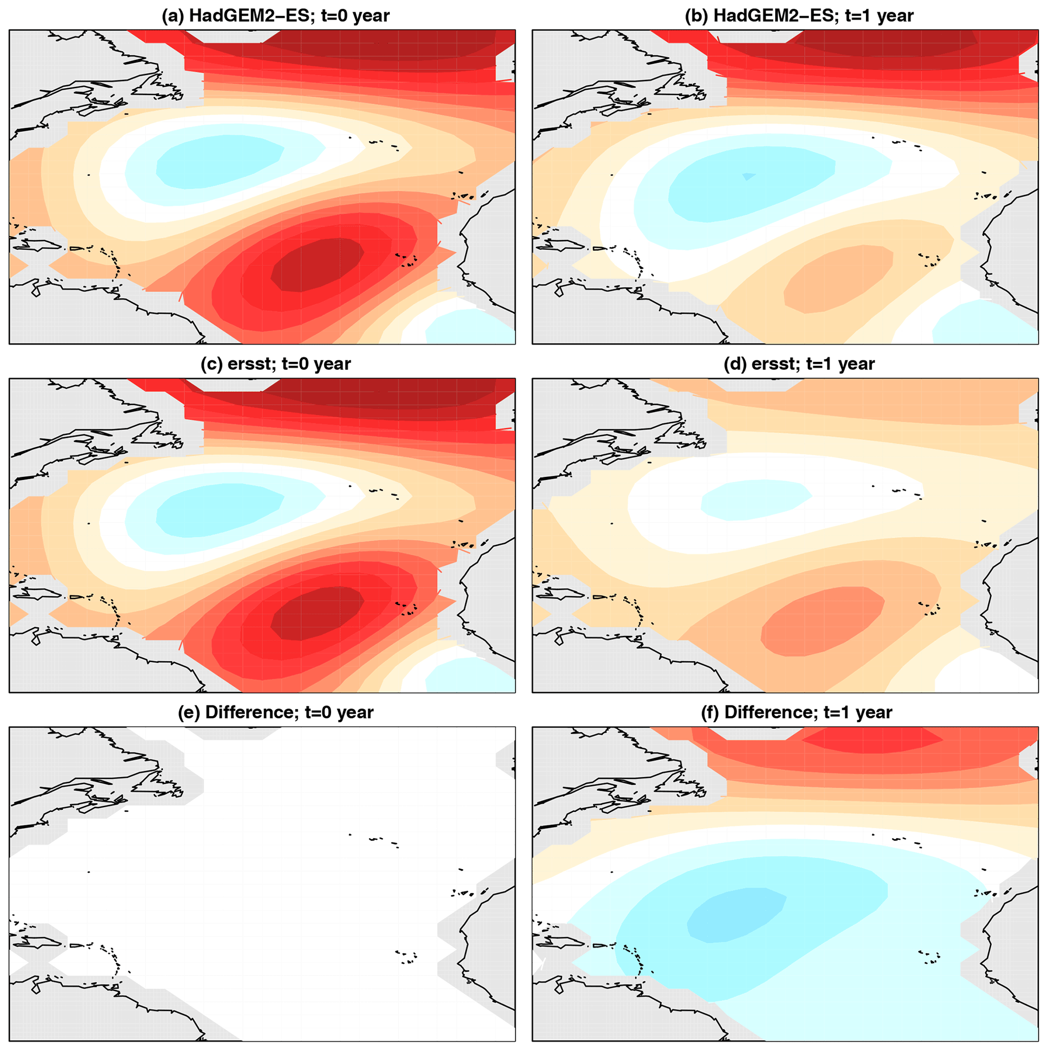
Figure 7The initial condition (a, c, e) that maximizes the difference in 1-year response of VAR models estimated from HadGEM2-ES (a, b) and ERSSTv5 (c, d). The resulting response of the initial condition is shown in (b), (d), and (f). Panel (e) shows panels (a) minus (c); panel (f) shows panels (b) minus (d). The color scale is the same across panels but is not shown because the amplitude is arbitrary for linear initial value problems.

Figure 8Same as Fig. 7 except for MIROC-ESM.
The leading difference-in-dynamics singular value s1 for each model is shown in Fig. 6. The model with the largest singular value is HadGEM2-ES. The results of difference-in-dynamics SVD are shown in Fig. 7. The left-hand-side panels show the initial condition pX,1 that maximizes the difference in responses (which is the same for the CMIP5 model and observations), and the right-hand-side panels show the response pY,1 of the respective VAR model to these initial conditions (along with the associated difference). We see that HadGEM2-ES gives a reasonable 1-year evolution over the subtropical–tropical areas but is much too persistent in the northernmost part of the domain compared to observations. To illustrate the diagnostic further, we show one more example. The results of difference-in-dynamics SVD for MIROC-ESM is shown in Fig. 8. As can be seen, the responses are dramatically different. Specifically, the VAR model from ERSSTv5 is predominantly a damping, whereas the VAR model from MIROC-ESM produces anomalies of the opposite sign in the North Atlantic.
This paper proposed techniques for optimally diagnosing differences between serially correlated, multivariate time series. The starting point is to assume each time series comes from a vector autoregressive model and then test the hypothesis that the model parameters are equal. The likelihood ratio test for this hypothesis was derived in Part II of this paper series, which leads to a deviance statistic that measures the difference in VAR models. However, merely deciding that two processes differ is not completely satisfying because it does not tell us the nature of those differences. For instance, a VAR can be viewed as a dynamical system driven by random noise, but do differences arise because of different dynamics, different noise statistics, or both? We show that the deviance between VAR models can be decomposed into two terms, one measuring differences in noise statistics and another measuring differences in dynamics (i.e., differences in AR parameters). Under suitable assumptions, the two terms are independent and have asymptotic chi-squared distributions, which leads to straightforward hypothesis testing. Then, the linear combination of variables that maximizes each deviance is obtained. One set of combinations identifies components whose noise covariances differ most strongly between the two processes. The other set of combinations effectively finds the initial conditions that maximize the difference in response from each VAR model.
The proposed method was applied to diagnose differences between annual-mean North Atlantic sea surface temperature variability between climate models and observations. The results show that differences in dynamics and differences in noise covariances both play a significant role in the overall differences. In fact, only one model was found to be consistent with observations. However, this consistency is not robust. In further analyses (not shown), we changed the half of observations used to diagnose differences and found that this model no longer was consistent with observations. In fact, no model was found to be consistent with both halves of the observational period. For half the models, the leading discriminant of noise variance explains 40 % or more of the deviance in noise covariances. For most models, the leading discriminant underpredicts the noise variance, and the associated spatial structures are highly model dependent. In contrast, models that have leading discriminants with too much noise variance tend to have similar spatial structures.
Discriminant analysis was also applied to identify differences in dynamics, or more precisely, differences in AR parameters. These discriminants can be interpreted as finding suitably normalized initial conditions that maximize the difference in response from the two VAR models. Examples from this analysis revealed dramatic errors in the 1-year predictions of some models. For instance, the VAR model trained on HadGEM2-ES gives realistic 1-year predictions at the mid to low latitudes of the North Atlantic but are much too persistent at the high latitudes. The VAR model trained on MIROC-ESM produces 1-year predictions with the wrong sign in the North Atlantic.
Although previous climate studies have diagnosed differences in variability using discriminant techniques (Schneider and Griffies, 1999; DelSole et al., 2011; Wills et al., 2018), the above procedure differs from previous analysis in important ways. Specifically, here discriminant techniques are applied to a measure of dissimilarity that has a simple significance test. This means that the dissimilarity measure can be tested for significance before embarking on a diagnosis of the dissimilarities. The simplicity of the test is a consequence of measuring dissimilarities of prewhitened variables rather than dissimilarities in the original, serially correlated variables. In general, prewhitened variables are closer to white noise than the original data, and hence their asymptotic distributions are simpler than those of the original process.
Diagnosing differences in dynamics leads to generalized SVD, which differs from the SVD used in previous studies to diagnose dynamics of linear inverse models (e.g., Penland and Sardeshmukh, 1995; Winkler et al., 2001; Shin and Newman, 2021). In particular, standard SVD uses the Euclidean norm to constrain the initial and final vectors, which yields singular vectors that depend on the coordinate system. This dependence might be averted by asserting a norm to be some physical quantity like energy or enstrophy, but these assertions usually have no compelling justification and lead to statistics with no simple significance test. In contrast, difference-in-dynamics SVD emerges from a rigorous statistical framework, and, as a result, it leads to simple significance tests, and the norms chosen for maximization are dictated by the statistical framework and lead to results that are independent of the arbitrary coordinate system.
One reason for diagnosing differences in stochastic processes is to gain insight into the causes of the differences. For instance, dissimilarities in noise processes indicate differences in the one-step prediction errors of the associated VAR models. Comparison of prediction errors may give clues as to the locations or processes that dominate the errors, which may be helpful for improving a climate model. Similarly, differences in dynamics indicate differences in the memory or in the evolution of anomalies between observations and climate models. The diagnostics derived here may give clues as to the physical source of the differences, which in turn may give insight into how to improve climate models.
This Appendix proves the key results of decomposing D1:2, namely, Eqs. (24) and (25). We begin with the eigenvalue problem Eq. (23). Let us collect the eigenvectors into the matrix
Recall that eigenvectors are unique up to a multiplicative factor, and hence we may normalize them such that . Because and are symmetric, the eigenvectors satisfy the following properties (see Seber, 2008, result 6.67):
where Θ is a diagonal matrix with diagonal elements . For each eigenvector qY,i, a time series can be computed from Eq. (19). The variates for all the eigenvectors may be collected into a single matrix as
Then, Eq. (19) implies
and this combined with Eqs. (9), (10), and (A2) implies that the associated covariance matrices are
Diagonal covariance matrices imply that the variates are uncorrelated and therefore independent under normality.
Because the eigenvectors are distinct and form a complete basis set, QY is non-singular, and we may define
where the first equality is a definition and the second equality follows from Eq. (A2). Multiplying Eq. (A3) on the right by and using Eq. (A4) yields
If the column vectors of are denoted as , then Eq. (A5) can be written equivalently as Eq. (24).
Importantly, the above decomposition also decomposes the deviance. To see this, note that Eqs. (A2) and (A4) imply
Substituting these expressions into Eq. (15) and using standard properties of the determinant yields
which is Eq. (25). This completes the proofs of Eqs. (24) and (25).
In this Appendix, we prove that the matrix defined in Eq. (11) can be decomposed as
where
and
Identity Eq. (B1) clarifies that D0:1 defined in Eq. (14) measures differences in AR parameters, because if , then D0:1 vanishes (because then Δ=0 and therefore ); otherwise, D0:1 is positive (because is positive definite). This identity will be needed in Appendix C.
Starting from the definition Eqs. (6)–(11), we note that the MSEs satisfy the standard orthogonality relations
It follows from these orthogonality relations that
Therefore, the MLE of Γ0 in Eq. (11) can be written equivalently as
where
To show that this Δ equals Eq. (B2), note that
To simplify notation, we define
Then,
Similarly, we have
Thus,
Similarly, we have
Adding these together, dividing by ν1+ν2, and returning to the original notation gives
which is Eq. (B2), as desired.
This Appendix proves the key results of decomposing D0:1, namely, Eqs. (31), (33), (34), and (35). Our starting point is the solution to the eigenvalue problem Eq. (28). Let the eigenvalues from Eq. (28) be and the associated eigenvectors be . The eigenvectors may be collected into the matrix QY, analogous to Eq. (A1). Furthermore, because the matrices in Eq. (28) are symmetric, the eigenvectors may be normalized to satisfy (see Seber, 2008, result 6.67)
where Λ is a diagonal matrix with diagonal elements . If the eigenvalues are distinct, then the eigenvectors form a complete basis set and QY is non-singular, and hence we may define
where the second equality follows from the first identity in Eq. (C1). Using Eq. (C2), the identity Eq. (C1) can be written equivalently as
Now, consider the Rayleigh quotient Eq. (27). The matrices and are related to each other through Eq. (B1). Substituting Eq. (B1) into Eq. (27) yields
where s2 is the Rayleigh quotient
Let denote the matrix square root of . Then, Eq. (C5) can be written equivalently as
where
and
A standard result in linear algebra states that extrema of Eq. (C6) are given by the eigenvectors of ΦTΦ or equivalently the singular vectors of Φ. Let the singular value decomposition (SVD) of Φ be
where U and V are orthogonal matrices and S is a diagonal matrix with non-negative diagonal elements called singular values. Because , maximizing s2 in Eq. (C6) is equivalent to maximizing λ in Eq. (27). Therefore, the squared singular values must equal the eigenvalues , and the eigenvectors must give the right singular vectors through Eq. (C7). Let be ordered from largest to smallest.
Comparing Eqs. (C8) and (C9), we can anticipate that U describes initial conditions, V describes differences in responses, and diagonals of S measure response amplitudes. To be more precise, define
Note that Eqs. (C2) and (C3) hold for the above definitions, as they should since the eigenvalue problem Eq. (28) and SVD Eq. (C9) perform the same decomposition. Furthermore, Eq. (C10) implies the additional identities
the first two of which give Eq. (32), and the last implies . However, Eq. (C9) can be rearranged into the form
which, after expanding QX and into column vectors, can be written equivalently as Eq. (31). Decomposition Eq. (C12) and the first two identities in Eq. (C11) are a weighted form of the generalized singular value decomposition (Abdi and Williams, 2010).
Just as the column vectors of V maximize the Rayleigh quotient Eq. (C6), the column vectors of U maximize
which is Eq. (35). In addition, the identity ΦTU=VST implies
which gives Eq. (34). An additional property of can be derived from the identity ΦTΦ=VS2VT, which implies
which in turn can be written equivalently as
This identity shows that Δ can be decomposed into a sum of terms involving pY,i without any cross terms. Finally, Eqs. (30) and (C4) imply
which shows that the SVD of Φ partitions the deviance into a sum of components ordered by their contribution to D0:1.
In this section, we prove that the eigenvalues from Eqs. (23) and (28) are invariant to invertible linear transformations of the form
where primes indicate transformed quantities and G is a square, non-singular matrix. Using straightforward matrix algebra, Eqs. (6)–(13) are transformed as
Substituting transformed quantities into the eigenvalue problem Eq. (23) yields
where the second line follows by substituting Eqs. (D3) and (D4), the third line follows by multiplying both sides on the left by the inverse of GT (which is possible because G is invertible), and the fourth line follows by defining
This shows that linear transformations do not affect the eigenvalues of Eq. (23), while they transform the eigenvectors as Eq. (D7).
Similarly, substituting transformed quantities into the eigenvalue problem Eq. (28) yields
By the same steps as above, this eigenvalue problem can be transformed to Eq. (28). This shows that the eigenvalues of Eq. (28) are invariant to invertible linear transformations. Because of Eq. (C4), it follows that the difference-in-dynamics singular values sj are also invariant to invertible linear transformations.
R codes for performing the statistical test described in this paper are available at https://github.com/tdelsole/Comparing-Time-Series (DelSole, 2022).
The data used in this paper are publicly available from the CMIP archive https://eprints.soton.ac.uk/194679/ (CMIP5, 2022).
Both authors participated in the writing and editing of the manuscript. TD performed the numerical calculations.
The contact author has declared that neither they nor their co-author has any competing interests.
The views expressed herein are those of the authors and do not necessarily reflect the views of this agency.
Publisher’s note: Copernicus Publications remains neutral with regard to jurisdictional claims in published maps and institutional affiliations.
We thank the World Climate Research Programme’s Working Group on Coupled Modelling, which is responsible for CMIP, and we thank the climate modeling groups for producing and making available their model output. For CMIP the U.S. Department of Energy’s Program for Climate Model Diagnosis and Intercomparison provides coordinating support and led development of software infrastructure in partnership with the Global Organization for Earth System Science Portals.
This research has been supported by the National Oceanic and Atmospheric Administration (grant no. NA20OAR4310401).
This paper was edited by Christopher Paciorek and reviewed by Raquel Prado and one anonymous referee.
Abdi, H. and Williams, L. J.: Principal component analysis, WIREs Comput. Stat., 2, 433–459, https://doi.org/10.1002/wics.101, 2010. a, b
Alexander, M. A., Matrosova, L., Penland, C., Scott, J. D., and Chang, P.: Forecasting Pacific SSTs: Linear Inverse Model Predictions of the PDO, J. Clim., 21, 385–402, https://doi.org/10.1175/2007JCLI1849.1, 2008. a
Anderson, T. W.: An Introduction to Multivariate Statistical Analysis, Wiley-Interscience, 675 pp., 1984. a, b
Box, G. E. P., Jenkins, G. M., and Reinsel, G. C.: Time Series Analysis: Forecasting and Control, Wiley-Interscience, 4th Edn., 746 pp., 2008. a
CMIP5: CLIVAR Exchanges – Special Issue: WCRP Coupled Model Intercomparison Project – Phase 5 – CMIP5, Project Report 56, CMIP5 [data set], https://eprints.soton.ac.uk/194679/ (last access: 7 May 2020), 2011. a
DelSole, T.: Stochastic models of quasigeostrophic turbulence, Surv. Geophys., 25, 107–149, 2004. a
DelSole, T.: diff.var.test.R, GitHub [code], https://github.com/tdelsole/Comparing-Time-Series, last access: 17 January 2022. a
DelSole, T. and Tippett, M. K.: Comparing climate time series – Part 1: Univariate test, Adv. Stat. Clim. Meteorol. Oceanogr., 6, 159–175, https://doi.org/10.5194/ascmo-6-159-2020, 2020. a
DelSole, T. and Tippett, M.: Statistical Methods for Climate Scientists, Cambridge University Press, Cambridge, 526 pp., 2022. a
DelSole, T. and Tippett, M. K.: Comparing climate time series – Part 2: Multivariate test, Adv. Stat. Clim. Meteorol. Oceanogr., 7, 73–85, https://doi.org/10.5194/ascmo-7-73-2021, 2021a. a
DelSole, T. and Tippett, M. K.: A mutual information criterion with applications to canonical correlation analysis and graphical models, Stat, 10, e385, https://doi.org/10.1002/sta4.385, 2021b. a
DelSole, T., Tippett, M. K., and Shukla, J.: A significant component of unforced multidecadal variability in the recent acceleration of global warming, J. Clim., 24, 909–926, 2011. a, b
Dias, D. F., Subramanian, A., Zanna, L., and Miller, A. J.: Remote and local influences in forecasting Pacific SST: a linear inverse model and a multimodel ensemble study, Clim. Dynam., 52, 1–19, 2018. a
Farrell, B. F. and Ioannou, P. J.: Stochastic dynamics of the midlatitude atmospheric jet, J. Atmos. Sci., 52, 1642–1656, 1995. a
Flury, B. K.: Proportionality of k covariance matrices, Stat. Prob. Lett., 4, 29–33, https://doi.org/10.1016/0167-7152(86)90035-0, 1986. a
Fujikoshi, Y., Ulyanov, V. V., and Shimizu, R.: Multivariate Statistics: High-dimensional and Large-Sample Approximations, John Wiley & Sons, 533 pp., 2010. a
Gottwald, G. A., Crommelin, D. T., and Franzke, C. L. E.: Stochastic Climate Theory, in: Nonlinear and Stochastic Climate Dynamics, edited by: Franzke, C. L. E. and O'Kane, T. J., 209–240, Cambridge University Press, https://doi.org/10.1017/9781316339251.009, 2017. a
Hogg, R. V.: On the Resolution of Statistical Hypotheses, J. Am. Stat. Assoc., 56, 978–989, http://www.jstor.org/stable/2282008 (last access: 3 May 2022), 1961. a, b
Hogg, R. V., McKean, J. W., and Craig, A. T.: Introduction to Mathematical Statistics, Pearson Education, 8th Edn., 746 pp., 2019. a, b
Huang, B., Thorne, P. W., Banzon, V. F., Boyer, T., Chepurin, G., Lawrimore, J. H., Menne, M. J., Smith, T. M., Vose, R. S., and Zhang, H.-M.: Extended Reconstructed Sea Surface Temperature, Version 5 (ERSSTv5): Upgrades, Validations, and Intercomparisons, J. Clim., 30, 8179–8205, https://doi.org/10.1175/JCLI-D-16-0836.1, 2017. a
Huddart, B., Subramanian, A., Zanna, L., and Palmer, T.: Seasonal and decadal forecasts of Atlantic Sea surface temperatures using a linear inverse model, Clim. Dynam., 49, 1833–1845, https://doi.org/10.1007/s00382-016-3375-1, 2016. a
Kim, S.-H. and Cohen, A. S.: On the Behrens-Fisher Problem: A Review, J. Educat. Behav. Stat., 23, 356–377, https://doi.org/10.3102/10769986023004356, 1998. a
Lütkepohl, H.: New introduction to multiple time series analysis, Spring-Verlag, 764 pp., 2005. a, b
Majda, A., Timofeyev, J., and Vanden-Eijnden, E.: Stochastic models for selected slow variables in large deterministic systems, Nonlinearity, 19, 769–794, 2006. a
Mardia, K. V., Kent, J. T., and Bibby, J. M.: Multivariate Analysis, Academic Press, 418 pp., 1979. a
Newman, M.: An Empirical benchmark for decadal forecasts of global surface temperature anomalies, J. Clim., 26, 5260–5269, 2013. a
Newman, M. and Sardeshmukh, P. D.: Are we near the predictability limit of tropical Indo-Pacific sea surface temperatures?, Geophys. Res. Lett., 44, 8520–8529, https://doi.org/10.1002/2017GL074088, 2017. a
Noble, B. and Daniel, J. W.: Applied Linear Algebra, Prentice-Hall, 3rd Edn., 521 pp., 1988. a
Penland, C.: Random forcing and forecasting using principal oscillation pattern analysis, Mon. Weather Rev., 117, 2165–2185, 1989. a
Penland, C. and Sardeshmukh, P. D.: The optimal growth of tropical sea-surface temperature anomalies, J. Clim., 8, 1999–2024, 1995. a, b
Scheffé, H.: Practical Solutions of the Behrens-Fisher Problem, J. Am. Stat. Assoc., 65, 1501–1508, https://doi.org/10.1080/01621459.1970.10481179, 1970. a
Schneider, T. and Griffies, S.: A Conceptual Framework for Predictability Studies, J. Clim., 12, 3133–3155., 1999. a, b
Seber, G. A. F.: A Matrix Handbook for Statisticians, Wiley, 559 pp., 2008. a, b, c
Shin, S.-I. and Newman, M.: Seasonal predictability of global and North American coastal sea surface temperature and height anomalies, Geophys. Res. Lett., 48, e2020GL091886, https://doi.org/10.1029/2020GL091886, 2021. a, b
Taylor, K. E., Stouffer, R. J., and Meehl, G. A.: An Overview of CMIP5 and the Experimental Design, Bull. Am. Meteorol. Soc., 93, 485–498, 2012. a
Vimont, D. J.: Analysis of the Atlantic Meridional Mode Using Linear Inverse Modeling: Seasonality and Regional Influences, J. Clim., 25, 1194–1212, https://doi.org/10.1175/JCLI-D-11-00012.1, 2012. a
Wills, R. C., Schneider, T., Wallace, J. M., Battisti, D. S., and Hartmann, D. L.: Disentangling Global Warming, Multidecadal Variability, and El Niño in Pacific Temperatures, Geophys. Res. Lett., 45, 2487–2496, https://doi.org/10.1002/2017GL076327, 2018. a, b
Winkler, C. R., Newman, M., and Sardeshmukh, P. D.: A Linear Model of Wintertime Low-Frequency Variability, Part I: Formulation and Forecast Skill, J. Clim., 14, 4474–4494, 2001. a, b, c
Zanna, L.: Forecast skill and predictability of observed North Atlantic sea surface temperatures, J. Clim., 25, 5047–5056, 2012. a
- Abstract
- Introduction
- Likelihood ratio test for differences in vector autoregressive models
- Partitioning the deviance statistic
- Diagnosing differences in noise processes
- Diagnosing differences in dynamics
- Application to North Atlantic sea surface temperatures
- Conclusions
- Appendix A: Decomposition of D1:2
- Appendix B: Decomposition of
- Appendix C: Decomposition of D0:1
- Appendix D: Invariance to linear transformation
- Code availability
- Data availability
- Author contributions
- Competing interests
- Disclaimer
- Acknowledgements
- Financial support
- Review statement
- References
- Article
(6676 KB) - Full-text XML
- Abstract
- Introduction
- Likelihood ratio test for differences in vector autoregressive models
- Partitioning the deviance statistic
- Diagnosing differences in noise processes
- Diagnosing differences in dynamics
- Application to North Atlantic sea surface temperatures
- Conclusions
- Appendix A: Decomposition of D1:2
- Appendix B: Decomposition of
- Appendix C: Decomposition of D0:1
- Appendix D: Invariance to linear transformation
- Code availability
- Data availability
- Author contributions
- Competing interests
- Disclaimer
- Acknowledgements
- Financial support
- Review statement
- References