the Creative Commons Attribution 4.0 License.
the Creative Commons Attribution 4.0 License.
 | 02 Feb 2023
Modeling general circulation model bias via a combination of localized regression and quantile mapping methods
Benjamin James Washington
Thomas L. Mote
General circulation model (GCM) outputs are a primary source of information for climate change impact assessments. However, raw GCM data rarely are used directly for regional-scale impact assessments as they frequently contain systematic error or bias. In this article, we propose a novel extension to standard quantile mapping that allows for a continuous seasonal change in bias magnitude using localized regression. Our primary goal is to examine the efficacy of this tool in the context of larger statistical downscaling efforts on the tropical island of Puerto Rico, where localized downscaling can be particularly challenging. Along the way, we utilize a multivariate infilling algorithm to estimate missing data within an incomplete climate data network spanning Puerto Rico. Next, we apply a combination of multivariate downscaling methods to generate in situ climate projections at 23 locations across Puerto Rico from three general circulation models in two carbon emission scenarios: RCP4.5 and RCP8.5. Finally, our bias-correction methods are applied to these downscaled GCM climate projections. These bias-correction methods allow GCM bias to vary as a function of a user-defined season (here, Julian day). Bias is estimated using a continuous curve rather than a moving window or monthly breaks. Results from the selected ensemble agree that Puerto Rico will continue to warm through the coming century. Under the RCP4.5 forcing scenario, our methods indicate that the dry season will have increased rainfall, while the early and late rainfall seasons will likely have a decline in total rainfall. Our methods applied to the RCP8.5 forcing scenario favor a wetter climate for Puerto Rico, driven by an increase in the frequency of high-magnitude rainfall events during Puerto Rico's early rainfall season (April to July) as well as its late rainfall season (August to November).
- Article
(1865 KB) - Full-text XML
- BibTeX
- EndNote


In general, island climates are distinctly difficult to characterize, with Puerto Rico being no exception. Puerto Rico is situated well within the belt of easterly trade winds. These winds carry seasonal weather, generally dry from December through March when sea-surface temperatures typically reach a minimum (Taylor et al., 2002; Comarazamy and González, 2008; Ramseyer and Mote, 2018) and wetter from April through November. The wet season is broken into two distinct periods: the early rainfall season (ERS; April–July), and the late rainfall season (LRS; August–November) (Angeles et al., 2010). While hurricanes are typically the most extreme events arising from these tropical waves, severe weather commonly occurs seasonally in Puerto Rico from less well developed systems. As a consequence of this, accurate short-term and long-term forecasting at the local scale is a particularly desirable objective for this island. The long-term forecasting of a single extreme event may not be feasible, but what is of particular interest in these long-term forecasts is the frequency and intensity of these extreme events.
Many studies have utilized dynamic downscaling (DD) and statistical downscaling (SD) techniques in an effort to accurately model Puerto Rico's future climate. Bhardwaj et al. (2018) and Bowden et al. (2021) employ high-resolution regional climate models (RCMs) to develop dynamically downscaled climate estimates across a 2 km grid in Puerto Rico. Ramseyer and Mote (2016) and Ramseyer et al. (2018, 2019) examine the utility of neural networks as a method for downscaling precipitation within Puerto Rico, while other studies (Khalyani et al., 2016; Van Beusekom et al., 2016; Miller et al., 2019) focus on the impacts of climate change on water availability in Puerto Rico using several downscaled products.
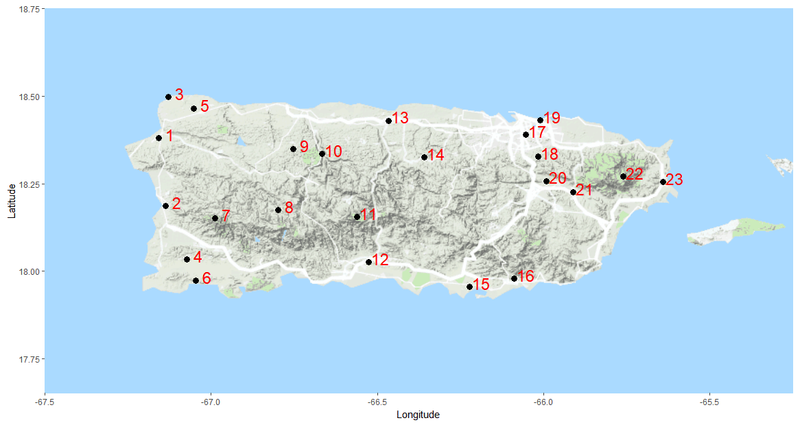
Figure 1The 23 weather stations of interest in Puerto Rico. This image was created using a combination of © Google Maps 2018, Kahle and Wickham (2013), and Wickham (2016).
In this study, we will employ SD in Puerto Rico in an effort to generate realistic daily temperature and precipitation data at 23 locations spanning Puerto Rico (Fig. 1). This work is unique in the fact that many prior Puerto Rico downscaling efforts do not focus on a suite of climate variables in tandem. A primary disadvantage of statistical downscaling is that the individually downscaled variables do not always act together in a physically consistent fashion, although some more recent approaches attempt to address this issue (Pierce et al., 2014; Cannon, 2018; Guo et al., 2019).
2.1 Global Historical Climatological Network data
The primary historical climate data are from the publicly available Global Historical Climatological Network (GHCN). Specifically, we are using the 23 weather stations listed in Table 1 (labeled west to east); refer to Fig. 1 for location.
Table 1The 23 GHCN weather stations of interest in Puerto Rico along with the proportion of missing observations (after cleaning – see Sect. 2.1.1 and 2.1.2) from 1 January 1978 through 31 December 2017.
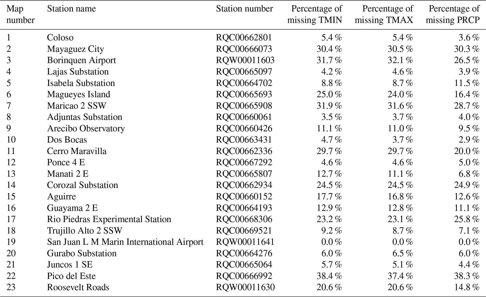
At each of these locations we have daily climate data consisting of maximum temperature (TMAX; ∘C), minimum temperature (TMIN; ∘C), and total precipitation (PRCP; mm). We focus on a 40-year time period from 1 January 1978 through 31 December 2017. Ideally, at each of our 23 stations we would have 14 610 observations (one for each day), but as is the case with many climate datasets, this dataset has many missing data points. We use the multivariate vector autoregressive time series methods of Washington and Seymour (2019) to infill missing values in this climate network. These methods extend the general multivariate autoregressive methods to allow for the inclusion of contemporaneous observations (as opposed to just lagged observations).
2.1.1 Temperature data cleaning
According to the National Weather Service (NWS), the hottest temperature ever recorded in San Juan, Puerto Rico, is 104 ∘F, while the minimum temperature ever recorded is 40 ∘F. These values have been cross-validated by the NCEI and/or by the State Climate Extremes Committee and determined to be valid. While these NWS temperature extrema should not be used as strict temperature cutoffs (any values outside of these bounds are removed), they still represent a plausible range of observed temperature values in Puerto Rico. By cross-referencing the monthly temperature boxplots reported in Fig. 2 and this NWS observed temperature range, it is apparent that there are a considerable number of potentially invalid temperature readings, thus exhibiting the need for quality control.
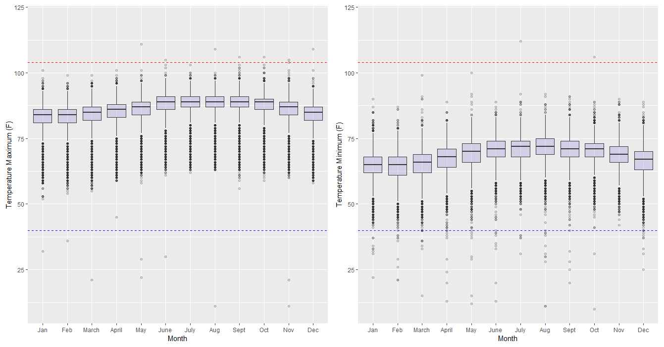
Figure 2 provides a representation of the seasonal cycle for temperature data across all 23 locations of interest; however, this general trend can be expected to vary from station to station. To identify temperature inaccuracies, all observations are first standardized across season and station as in Lund et al. (1995) and Washington et al. (2019). Suppose represents our daily temperature series at time t, for station j, in month ν, where N indicates the total sample size. Then, borrowing notation and terminology from Washington et al. (2019), the seasonally standardized anomaly (SSA) time series is constructed as in Eq. (1).
Here, represents the SSA value at time t, station j, and month ν; denotes the station j, month ν mean; and denotes the station j, month ν standard deviation. With the seasonally standardized temperature readings, inaccurate values may be more easily detected. Figure 3 displays the daily temperature maxima from 1 January to 31 December 1993 (left panel) and the corresponding SSA time series (right panel) for the Adjuntas Substation weather station (Location 8 in Fig. 1).
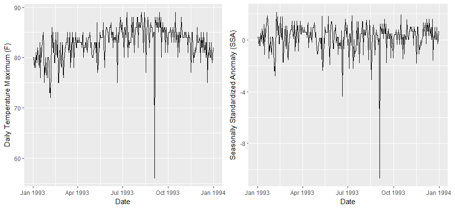
In Fig. 3, one clearly incorrect value can be observed on 3 September 1993, although there are possibly more incorrect values over this calendar year (in particular, 20 June). Suspected inaccuracies can be more easily observed in the right panel of Fig. 3 as they have been seasonally standardized. We use an automated temperature verification method which relies on a preliminary examination of the SSA series to flag anomalous temperatures. These flagged temperatures are then examined more closely.
-
Designate any observation with an absolute SSA value that is larger than 4 as a flagged value, the validity of which must be examined more closely.
-
Extract an 11 d interval of temperature readings within 5 d on either side of the flagged observation for all 23 weather stations. For example, 29 August to 8 September is the 11 d window surrounding the flagged value on 3 September 1993, from Fig. 3. These observations are then used to estimate the distribution of SSA values across this 11 d window.
-
Finally, if the flagged SSA value is more than 5.5 standard deviations away from the mean SSA value in this 11 d window, then the flagged temperature is recorded as not available (NA). The 5.5 standard deviation cutoff, though arbitrary, was chosen after examining the number of flagged observations from several potential cutoffs between 3 and 6 standard deviations.
This process not only allows one to identify potential outliers quickly (Item 1), but also provides a screening method to examine the validity of these potential outliers more closely (Item 2) and a threshold for acceptance–rejection (Item 3). By selecting an 11 d window around a flagged observation (Item 2), we allow for the possibility of a brief hot spell or cold spell. For example, it may be the case that a flagged observation (|SSA, Item 1) may be unexpected when compared to the entire 40-year time frame but may not be unexpected when compared to its 11 d time window.
After the screening was completed, 128 of the 933 flagged TMAX values were changed to NA, and 235 of the 855 flagged TMIN values were changed to NA. Finally, if a TMAX value is less than or equal to the corresponding TMIN value, both of the values are reported as NA. Altogether, these temperature quality control efforts omitted 252 TMAX and 359 TMIN recorded values. Combined with pre-screening missing values, this brings our total TMAX and TMIN missing values to 52 064 (15.5 % missing) and 52 886 (15.7 % missing), respectively.
2.1.2 Precipitation data cleaning
Precipitation quality control is particularly challenging in the tropics where isolated warm-water processes can drop large amounts of rain very quickly. Nesbitt et al. (2006) found that these isolated convective storms contributed a larger proportion of the total precipitation in the eastern Caribbean than larger-scale systems did. Furthermore, precipitation data are commonly zero-inflated and right-skewed, suggesting a need for an alternative cleaning mechanism (i.e., a seasonal standardization may not be appropriate for zero-inflated precipitation data). As was done with temperature, we identify and cull precipitation anomalies by examining them both spatially and seasonally. The quality control process is detailed below.
-
For each month, identify the largest 0.5 % of precipitation totals as flagged observations to be examined more closely.
-
For each flagged value, extract all 23 PRCP observations, representing each weather station on the given day.
-
If the flagged PRCP observation is more than 4 standard deviations away from the mean PRCP value on this day, then the precipitation value is rejected and recorded as NA.
Of the 1431 flagged precipitation observations (determined by taking the largest 0.5 % of each month's precipitation totals, Item 1), 158 of these were converted to NA as a result of the method described above for a total of 45 890 missing observations (13.7 % missing).
2.2 General circulation model data
We restrict ourselves to two common radiative forcing scenarios: RCP4.5 and RCP8.5 – that is, 4.5 and 8.5 W m−2 of additional radiative forcing beyond what the Sun is contributing. We are using data from the most recently completed Coupled Model Intercomparison Project at the time of this research: CMIP5 (however, now CMIP6 has been completed). In the CMIP project, ensemble model runs (or realizations) are named using what is referred to as the RIP nomenclature: R for realization (the starting point), I for initialization (initial model parameters at the beginning of the “burn-in” period), and P for physics (quantifiable atmospheric relationships), followed by an integer (Taylor et al., 2011, 2012). This study uses the first ensemble number (denoted: r1i1p1) for each of the three models (Table 2) to compare general circulation model (GCM) projections from two forcing scenarios (RCP4.5 and RCP8.5). Within each model, a fixed ensemble member allows for historical data to join seamlessly with the corresponding future projections (Taylor et al., 2011).
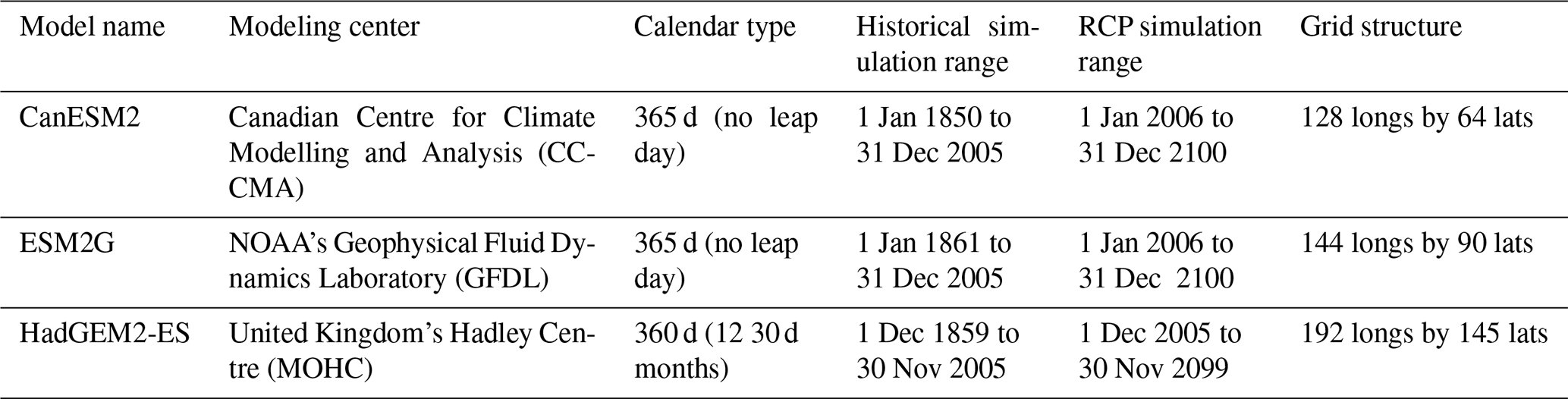
For each of the three climate models listed within Table 2 below, we have three separate data sources: simulation data using historical radiative forcing conditions and two future emission scenarios (RCP4.5 and RCP8.5). The variables of interest include daily average precipitation flux (kg m−2 s−1), daily minimum near-surface air temperature (K), and daily maximum near-surface air temperature (K). Although the temporal resolution (daily data) is consistent, the calendar type, spatial resolution, and temporal extent may differ across climate centers. The grid structure and temporal extents for each model are reported below.
Table 2The grid structure and temporal extents of each of the three GCMs utilized in this study.
Because this work is focused on Puerto Rico, we may greatly reduce the size of our GCM data. Figure 4 displays the CanESM2 grid structure surrounding Puerto Rico. Only coordinates which fall inside of the bounding box (highlighted in red) are retained in the reduction. As these models have their own spatial resolutions, the number of locations retained will vary (see Fig. A1 (GFDL-ESM2G) and Fig. A2 (MOHC-HadGEM2-ES) in Appendix A).
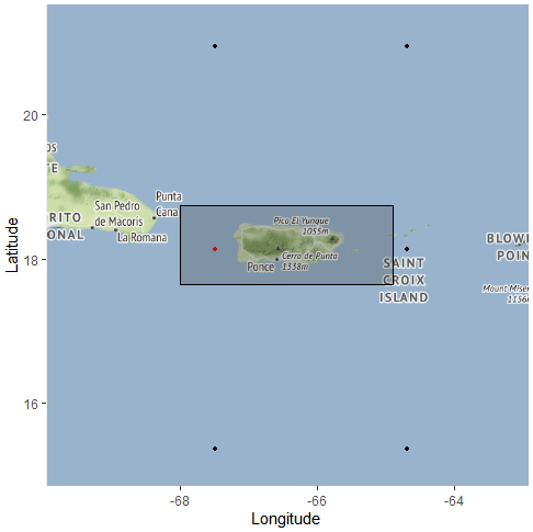
Figure 4The bounding box for which GCM coordinates are kept (latitudes range from 17.65 to 18.75∘, and longitudes range from −68.00 to −64.90∘). The CanESM2 location inside the box (red) is kept, while CanESM2 locations outside the box (black) are not kept. This image was created using a combination of © Google Maps 2018, Kahle and Wickham (2013), and Wickham (2016).
Many Caribbean downscaling methods used in climatology are applied to univariate time series and neglect dependence between variables (Cannon, 2018). Clearly, there is a strong correlation between daily minimum and maximum temperatures. For this reason, multivariate downscaling methods should be applied. To this end, we present a combination of ideas from Jeong et al. (2012a, b) to downscale climate data at K=23 locations simultaneously. Jeong et al. (2012a) employs a two-part multivariate multisite statistical downscaling model (MMSDM): (1) a multivariate multiple linear regression (MMLR) model combined with (2) a spatially correlated stochastic component to downscale maximum and minimum temperatures at K=9 weather stations in southern Quebec. In Jeong et al. (2012b) the MMSDM model is used to downscale precipitation probability and precipitation amount.
For each station (), we consider three predictands: daily temperature maximum (TMAXk), daily temperature minimum (TMINk), and daily total precipitation (PRCPk). As accurate forecasting of future precipitation behavior is so critical in this region, we decompose PRCPk into two separate variables: probability of precipitation occurrence (POCk) and precipitation amount (PAMk). POCk is coded as 1 for a rainy day (a day having more than 1 mm of rain) or a 0 for a dry day (Ben Alaya et al., 2014). In addition to this, many studies have found precipitation amounts to be gamma-distributed (Yang et al., 2005; Mattingly et al., 2017). To combat this right skew, we log-transform precipitation amount prior to downscaling: LogPAM), where designates the time (day). We add a small positive value to PAMtk in order to log-transform days with no precipitation; the value 1 preserves zeros: (ln(1)=0).
Final precipitation values are generated by drawing a single uniform random number for each day, , and comparing this uniform draw to all of the POCtk values (there should be 23 of them in our example) on day t. If ut<POCtk, it will be deemed a rainy day at station k; otherwise, it will be deemed a dry day at station k. For rainy days, final precipitation amounts will be generated by back-transforming LogPAMtk values. We define the T×M dimensional (M=4K) response matrix Y grouping all T×1 predictand vectors (TMAXk, TMINk, POCk, and LogPAMk) as follows.
Define XT×l to be the design matrix containing l−1 predictor variables. The exact dimensions of X will depend on the number of GCM locations retained and are noted in Sect. 5. The MMLR model can be expressed via
where E is the residual matrix. The parameter matrix β can be estimated via the standard ordinary least-squares (OLS) estimator: . The MMLR predicts only the deterministic components which are explainable by a linear relationship between the predictands and the GCM data (the predictor variables). The MMSDM introduced by Jeong et al. (2012a) utilizes the MMLR model as a means of simulating deterministic climate series from coarse-scale GCM data. The MMLR is unable to reproduce the spatial correlation observed between each location adequately.
In order to correct for the spatial bias, spatially correlated random noise is added to the simulated deterministic climate series. This random noise is generated from a multivariate normal distribution. The multivariate covariance matrix is estimated from the error matrix E. By definition,
where . Define to be the cross-correlated error matrix used as a means of more adequately capturing the spatial correlation among weather stations. Finally, define Σ=SCS, where S is a diagonal matrix containing the estimated standard deviations of each column of the residual matrix, E, and C represents the correlation matrix of the residual matrix, E. Now, this stochastic component is added directly to the deterministic component to obtain spatially correlated estimates of the predictands:
Raw GCM output frequently contain systematic error or bias (Thrasher et al., 2012). In many cases, the errors in GCM simulations relative to historical observations can be quite large (Ramirez-Villegas et al., 2013). Downscaling exists not only to refine GCM output both spatially and temporally, but also to quantify and correct these systematic errors. There are numerous bias-correcting methods (Müller et al., 2011; Cannon, 2018), and no one method is universally accepted as optimal in all situations. GCM bias may vary spatially, temporally, and across model, variable, and season. In addition to this, GCMs are known to have a “drizzle problem” where too many low-magnitude rain events are projected to occur as compared with historical GHCN observations (Chen et al., 2021; Gutowski et al., 2003).
Many downscaling methods are able to capture and correct at least some of a GCM's bias through the use of transfer functions (Winkler et al., 1997). However, different transfer functions do not uniformly capture GCM bias. Furthermore, bias-correction techniques may be applied to the raw GCM data prior to downscaling or applied to the generated climate data after downscaling. When applying a post hoc bias correction, one must assume that the spatial and temporal correlations of the raw downscaled data are preserved after any adjustments to one or more variables in the network. In this research, we introduce post hoc bias-correction methods where bias is estimated via a combination of locally estimated scatterplot smoothing (LOESS) methods (Cleveland et al., 2017) and quantile mapping.
Quantile mapping (QM) is a commonly used technique to remove or diminish systematic GCM error (Park et al., 2012; Thrasher et al., 2012; Lafon et al., 2013; Maraun, 2013). There are several criticisms of quantile mapping. Perhaps most notably, standard QM methods adjust a climate variable's distribution as a whole and do not explicitly account for spatial, temporal, nor multivariate aspects of the predictands (Maraun, 2016). Put differently, standard quantile mapping inherently assumes that the bias magnitude is constant across space and time (or season) and, in a multivariate setting, does not significantly impact the correlation between downscaled climate variables. For this reason, much of the current literature extends standard quantile mapping to allow bias to vary seasonally. For instance, Thrasher et al. (2012) utilize a 31 d window (center day ±15 d) to construct the cumulative distribution functions (CDFs). Wood et al. (2002) utilize a monthly bias correction so that each month is assumed to have its own bias magnitude. Despite its criticisms, QM remains a highly regarded and widely used GCM bias-correction method. We propose a similar extension to standard quantile mapping techniques that allows for a continuous seasonal change in bias magnitude to be estimated using LOESS smoothing splines.
4.1 LOESS quantile mapping
Through motivating examples using one generation of downscaled CanESM2 precipitation data (as precipitation is often most difficult to characterize), we introduce and discuss our novel bias-correction technique we call LOESS quantile mapping or LQM. LQM accounts for a bias which may vary seasonally by combining elements of LOESS regression and quantile mapping. LOESS methods (Cleveland et al., 2017) approximate a “best-fitting” smoothed scatterplot curve through a series of weighted regressions. The curve is estimated using a local neighborhood of points surrounding a location x, weighted by their distance from x: . The local neighborhood is chosen using a smoothing parameter, α, where : α indicates the proportion of data considered to be neighboring x. In this section, we apply these methods to the raw LogPAMk (log precipitation amount) values, but these methods will also be used to correct temperature bias. Figure 5 displays the estimated CDFs of the observed (red), fitted (green), downscaled RCP4.5 (blue), and downscaled RCP8.5 (purple) log precipitation distributions.
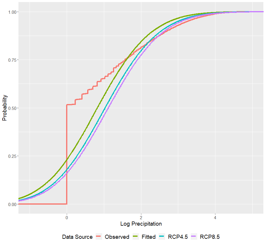
A standard QM procedure maps the fitted CDF (green curve in Fig. 5) onto the observed CDF (red curve in Fig. 5). By comparing these two curves, we can see that the MMSDM downscaling also falls victim to the “drizzle problem” mentioned earlier: low-magnitude rain events are overpredicted, and high-magnitude rain events are underpredicted. In the top panels of Fig. 6, we plot the quartiles of the observed (red) and fitted (cyan) log precipitation as a function of Julian day. Recall that raw fitted log precipitation values may be negative. In the bottom panels, we plot the differences between the two curves (observed−fitted) along with a LOESS smoothing spline.
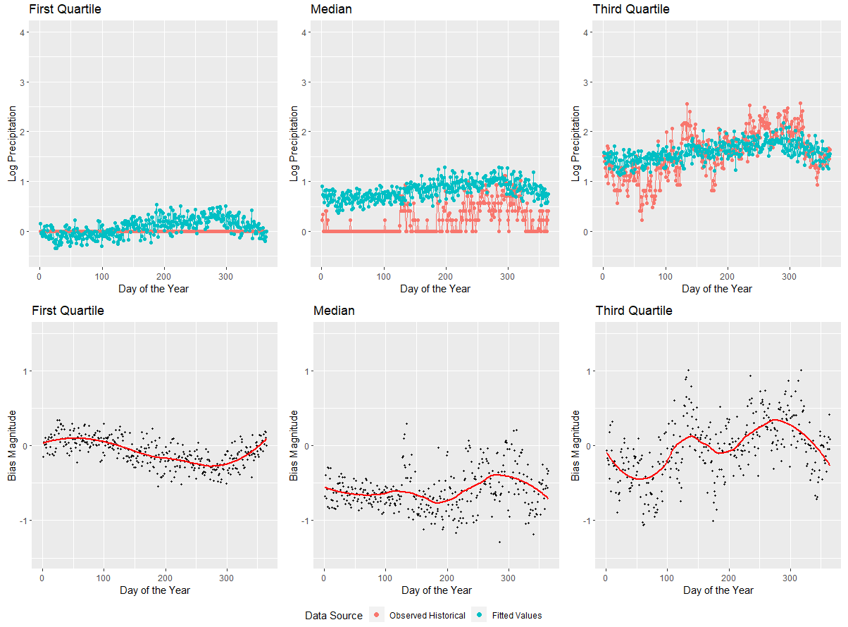
Figure 6Quartiles of fitted (cyan) and observed (red) log precipitation (mm) as a function of Julian day (top panel) using Canada's CanESM2. The differences between the observed and fitted precipitation along with a LOESS smoothing spline with smoothing parameter λ=0.50 (bottom panel). This figure was created using Wickham (2016).
Perhaps bias is negligible across season for lower-magnitude rain events because a negative bias-correction factor in LogPAMk may not heavily affect back-transformed PRCPk (first two columns of Fig. 6). However, the bias associated with larger precipitation events (daily third-quartile rain events, for example) is clearly dependent on season (third column of Fig. 6). Fitted precipitation values in the third quartile of daily precipitation totals that fall around day 50 (mid-February) are overpredicted, whereas similar third-quartile rainfall events that occur around day 140 (mid-May) or day 275 (the beginning of October) are underpredicted. These under-fitted high-magnitude rain events in May and October are consistent with the Caribbean's distinct bimodal rainy season (Chen and Taylor, 2002; Taylor et al., 2002; Angeles et al., 2010; Ramseyer and Mote, 2018). The LQM methodology is laid out below.
-
Estimate the percentiles of the observed values, , and fitted values, , of a downscaled random variable, X (log precipitation, LogPAMk), at specified steps in probability, p (0.01), as a function of season, ν (day).
-
Estimate the bias magnitude as a function of probability and season: , where , and N is the number of unique seasons (365).
-
Using a localized regression (LOESS) or some other smoothing mechanism, fit a smooth curve through the estimated bias scatter: l(B(p,ν)). This smoothed-bias estimate will be the bias-correction factor for a given percentile, p, and a given day, ν.
-
If the estimated percentile of a value of the random variable X, say xp,ν, falls exactly at a step increment of the percentile (), then simply correct this value using the estimated bias for that percentile and day: , where indicates the corrected value.
-
More often than not, the estimated percentile of a single value of the random variable X will not fall exactly at a step increment of p. In this case, round the estimated percentile to a user-specified resolution (three decimals) and linearly interpolate between its two nearest step increments – see graphical example in Figs. 7 and 8.
Take, for example, a fitted log precipitation value on day ν. Suppose its rounded percentile is p=0.804 when compared to all other fitted log precipitation values on day ν. Figure 7 displays the bias magnitudes of the 80th (red) and 81st (cyan) daily percentiles of log precipitation.
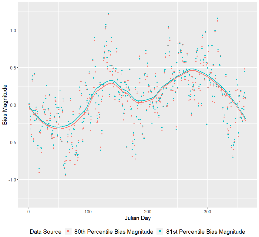
In Fig. 8, we expand the 100 d period from day ν=101 (11 April) to day ν=200 (19 July). On day ν=139 (19 May), we graphically display the bias magnitude interpolation process. Dashed lines indicate bias corrections for fitted values located between 80th (red) and 81st (cyan) percentiles of log precipitation on day ν=139. The solid purple line indicates the bias-correction factor for a fitted log precipitation on 19 May (Julian day ν=139) whose percentile (rounded to three decimals) is p=0.804. The intersection of the solid purple line and the solid black line represents the estimated bias-correction factor for 19 May.
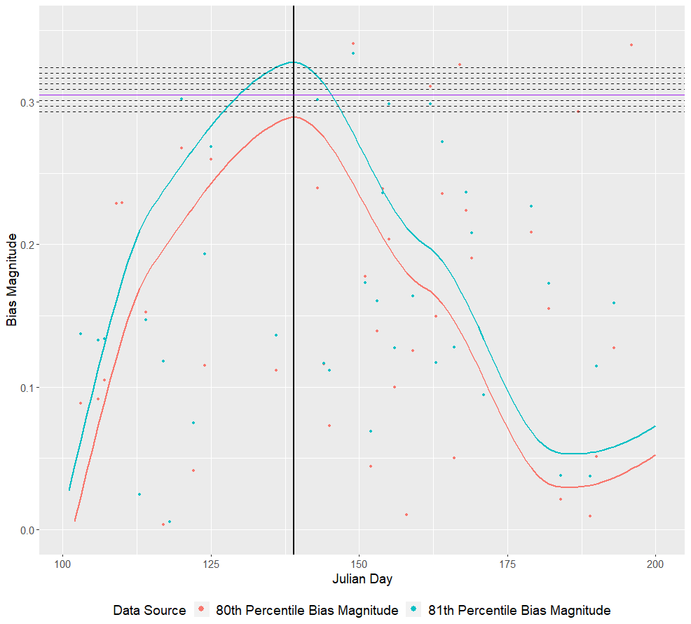
Figure 8Graphical display of the interpolation process for fitted log precipitation (mm) values, with percentiles falling between p=0.80 and p=0.81 on 19 May (day ν=139, vertical black line). The red and cyan curves represent the 80th and 81st percentiles of log precipitation as a function of day, respectively. This figure was created using Wickham (2016).
Figure 9 displays CanESM2 mean precipitation (mm) across all 23 stations from 1980 to 2005 as a function of Julian day for the true historical GHCN observation values (red), raw fitted values (green), LQM bias-corrected values (blue), and QM bias-corrected values that do not allow bias to vary as a function of season (purple) at three different LOESS bandwidths and two different step sizes. We can see two distinct peaks in precipitation corresponding to the ERS and the LRS. As one might expect, and as many other authors have observed (Thrasher et al., 2012; Wood et al., 2002), we see that the QM method that does not account for seasonal change is unable to adequately match the ERS and LRS rainfall peaks. Although there is not much difference between step sizes p=0.01 and p=0.001, we do observe substantial differences for different smoothing parameters. As intuition would indicate, a smaller smoothing parameter is more able to capture extreme precipitation.

Figure 9Average precipitation (mm) across all 23 stations from 1980 to 2005 as a function of Julian day for observed values (red), raw fitted values (green), LQM bias-corrected values (blue), and QM bias-corrected values (purple) using Canada's CanESM2 model at three different LOESS smoothing spans and two different step sizes. This figure was created using Wickham (2016).
4.2 LQM and QM model fit
In Sect. 4.1, we introduced LQM through motivating examples using CanESM2 precipitation data. In this section, we will compare results of LQM and QM on CanESM2 temperature and precipitation data. In Fig. 10, we plot the average LQM RMSE (red, smoothing parameter: 0.05) and QM RMSE (cyan) as a function of Julian day for TMAX (left), TMIN (middle), and PRCP (bottom right).
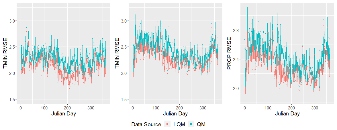
While LQM RMSE does not always outperform QM RMSE by a large margin, it is slightly lower overall. However, LQM (using smoothing parameter 0.05) does clearly outperform QM when we examine daily mean fitted values. Figure 11 plots the average TMAX (left), TMIN (middle), and PRCP (right) across all 23 stations from 1980 to 2005. We observe that the LQM bias-corrected fitted values (green) tend to match up to the true historical GHCN observations (red) better than the QM bias-corrected fitted values do (blue). LQM is clearly more able to mimic the observed historical (GHCN) seasonal cycle for temperature (Fig. 11). Furthermore, the LQM bias-corrected precipitation is more able to capture the ERS and LRS peaks in mean rainfall.
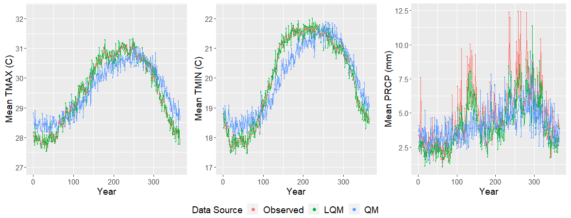
Figure 11Average TMAX (left), TMIN (middle), and PRCP (right) across all 23 stations from 1980 to 2005. The true historical GHCN observations are plotted in red, while the LQM bias-corrected fitted values and QM bias-corrected fitted values are plotted in green and blue, respectively. This figure was created using Wickham (2016).
In this section, we discuss the results of statistical downscaling efforts in Puerto Rico using the combination of our MMSDM methodology described in Sect. 3 with our LQM bias-correction methods of Sect. 4. We focus on results from the Canadian Centre for Climate Modelling and Analysis' CanESM2. Figures and tables generated for the US GFDL's ESM2G and the UK Hadley Centre's HadGEM2-ES can be found in Appendices B and C, respectively.
5.1 CCCMA's CanESM2 downscaled climate
Only one CanESM2 location is used to generate a downscaled climate in Puerto Rico (Fig. 4). The MMSDM downscaled climate estimates are derived from Eq. (5): , where contains the downscaled climate estimates, X34 675×4 contains the raw GCM climate projections, indicates the estimated parameter matrix, and H34 675×92 is a matrix of spatially correlated stochastic noise. The MMSDM model is trained using 26 years of historical observations (1980–2005) from the GHCN. Leap days, which are intentionally excluded in these methods, can be reasonably interpolated using a neighborhood of observations surrounding 29 February; however, we do not dwell on the generation of leap day climate here.
5.1.1 Temperature
Table 3 reports the extrema and deciles of historical and downscaled daily temperature maxima (∘C, top panel) and daily temperature minima (∘C, bottom panel). The extrema and deciles of the downscaled temperature maxima tend to be between 0–2 ∘C warmer than historical GHCN observations, while the extrema and deciles of the downscaled temperature minima tend to be between 1–3 ∘C warmer than historical observations. The extrema on the bottom-most ends of these distributions are lower that what might typically be expected in Puerto Rico, even at its highest elevations. These downscaled values are likely the result of inaccurate GHCN values that slipped through our culling process. We note that the occurrence of temperature minima between 1–3 ∘C is extremely rare (literally on the scale of a handful of times across 23 locations spanning Puerto Rico in the upcoming century).
Table 3Maximum daily temperature extrema and deciles (∘C, top panel) and minimum daily temperature extrema and deciles (∘C, bottom panel) for the observed historical (GHCN) climate, the downscaled RCP4.5 climate, and the downscaled RCP8.5.
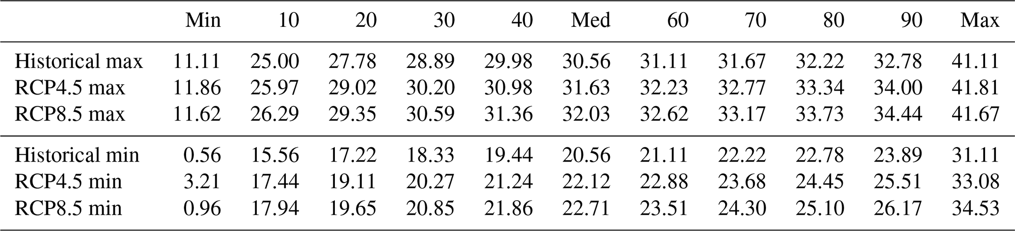
Figure 12 displays the CanESM2-estimated mean daily maximum temperature (left panel) and daily minimum temperature (right panel) as a function of year (1980–2100). We note that the subsequent plots may depict a small gap between the observed GHCN time series and the downscaled projections. This is merely an artifact of a GCM's “spin-up” period which represents a random realization of internal variability associated with its forcings and, therefore, may not perfectly align with GHCN observations. RCP4.5 projections indicate an increase in mean temperature that tapers off between 2050 and 2075, while RCP8.5 projects increasing maximum temperatures that continue to grow through 2100. These patterns are likely directly attributed to the greenhouse gas emissions exhibited by each forcing scenario. By 2100, maximum temperatures are projected to increase between 1.5–3 ∘C, on average (across all 23 locations), while minimum temperatures are projected to increase between 2–3.5 ∘C, on average.
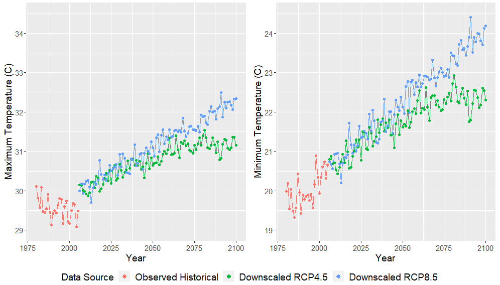
Figure 12CanESM2 mean daily maximum (left panel) and minimum (right panel) temperature (∘C) as a function of year. Observed historical GHCN data from 1980–2005 are plotted in red, while downscaled RCP4.5 and RCP8.5 temperatures from 2006–2100 are plotted in green and blue, respectively. This figure was created using Wickham (2016).
These observations are consistent with a large number of other downscaling works focused on the Caribbean (Centella et al., 2008; Harmsen et al., 2009; Campbell et al., 2011; Stennett-Brown et al., 2017). Because minimum temperature is expected to increase at a faster rate than maximum temperature, the average day will not only become warmer, but it will also observe a narrower range of diurnal temperatures. Both Biasutti et al. (2012) and Jennings et al. (2014) note a similar decrease in diurnal temperature variability throughout the Caribbean and Gulf of Mexico.
5.1.2 Precipitation
There is an overwhelming consensus of literature showing agreement that increasing greenhouse gas emissions will directly contribute to global warming (Lashof and Ahuja, 1990; Satterthwaite, 2008; Meinshausen et al., 2009). In a tropical climate, it is likely that temperature rise will be accompanied by an increase in specific humidity. Despite this, precipitation is likely to increase in some regions and decrease in others (Biasutti et al., 2012) making precipitation even more difficult to forecast. Within the Caribbean, recent literature tends to favor drying conditions, although some literature does provide conflicting opinions. Bowden et al. (2021), Campbell et al. (2011), and He and Soden (2017) all note a general drying pattern for Puerto Rico and its surrounding islands. Biasutti et al. (2012) note a 30 % decrease specific to spring and summer rainfall. Girvetz et al. (2009) and Meehl et al. (2007) project a decrease in Puerto Rico's annual precipitation, somewhere between 10 % and 30 %. Magrin et al. (2007), from the Fourth Assessment Report of the IPCC, project Latin America's annual precipitation to change anywhere from −40 % to +10 %. Cashman et al. (2010) find that the Caribbean will exhibit drying trends throughout the spring, summer, and fall; however, they project increased precipitation during the winter months, while Angeles et al. (2007) project a wetter climate for the Caribbean through 2050, driven heavily by increased rainfall during the rainy season, most likely a result of rising sea-surface temperatures which bolster large storm systems, potentially leading to an increase in the scale of extreme precipitation events.
While there may not be a clear consensus about projected annual Caribbean rainfall at the end of the century, there seems to be majority agreement within the literature that the Caribbean will exhibit increased variability in precipitation in the future. Many studies project an increased number of consecutive dry days, consistent with a lengthening of the dry season (Campbell et al., 2011; Biasutti et al., 2012). An increased number of consecutive dry days may have dire effects, not only on Puerto Rico's tropical ecosystem, but also on the water needs of the general public, who, being an island nation, rely heavily on consistent rainfall. Many other studies project an increase in the frequency and magnitude of extreme rainfall events (Magrin et al., 2007; Lintner et al., 2012; Ramseyer and Mote, 2016; Ramseyer et al., 2018, 2019), which have been shown in the recent past to have catastrophic and lasting effects on the island.
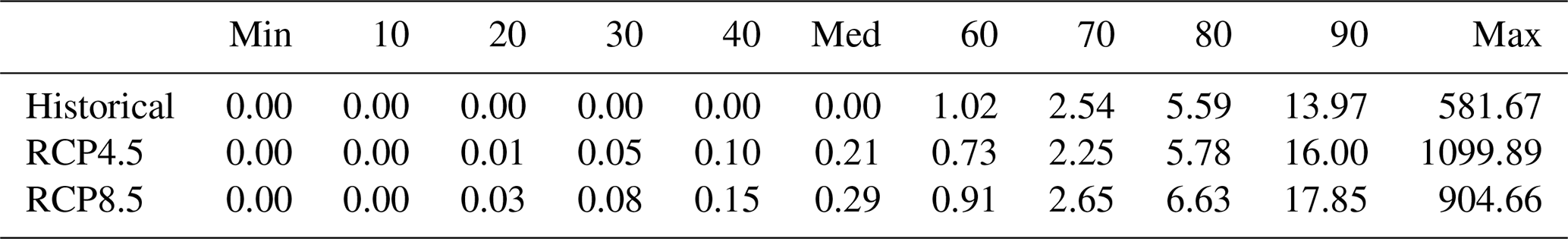
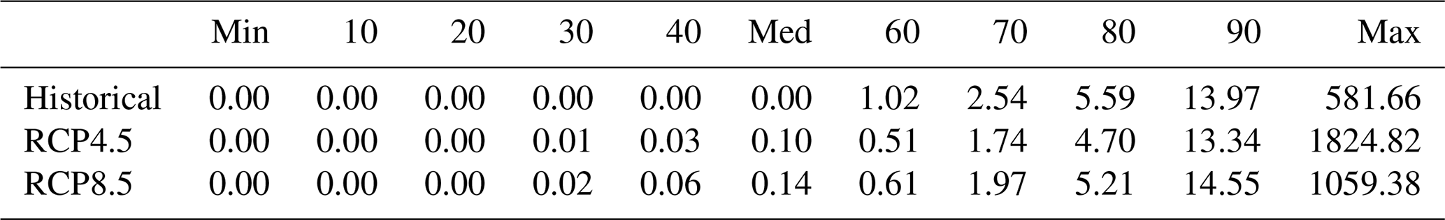
Table 4 displays the extrema and deciles of historical daily precipitation (mm) and projected daily precipitation (mm). The 60th percentiles (and the 70th percentile for RCP4.5) are smaller than those of the historical precipitation data. This suggests a diminishing number of small rainfall events in a future Puerto Rican climate. Furthermore, the 80th percentile, 90th percentile, and maximum projected rainfall events are all larger than those of the corresponding historical rainfall data, suggesting that Puerto Rico will begin to experience an increased number of large precipitation events.
Table 4CanESM2 daily total precipitation (mm) quantiles for the observed historical (GHCN) climate (1980–2005), the downscaled RCP4.5 climate (2006–2100), and the downscaled RCP8.5 climate (2006–2100) across all 23 locations.
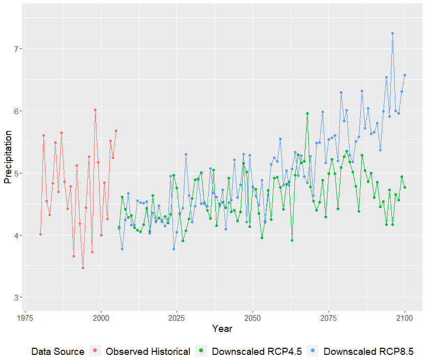
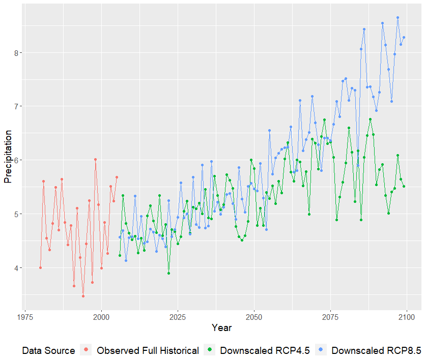
Despite an apparent reduction in low-magnitude precipitation events, the CanESM2 clearly favors a wetter future climate across Puerto Rico (Fig. 13), on average, across all stations. The RCP4.5 forcing scenario predicts an increase in average daily rainfall of around 1.5 mm, whereas the RCP8.5 projects an increase of nearly 3.5 mm by 2100.
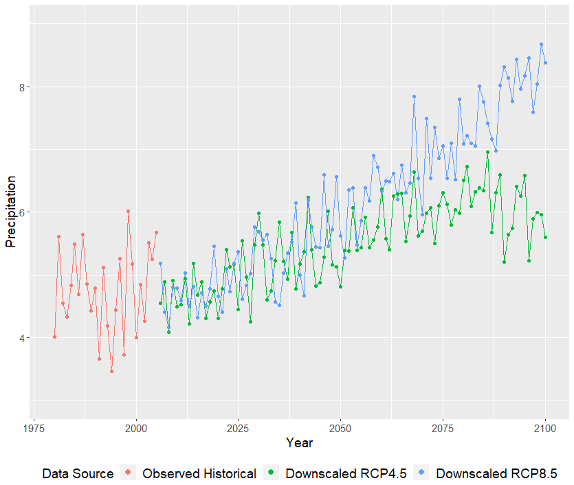

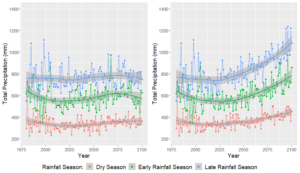
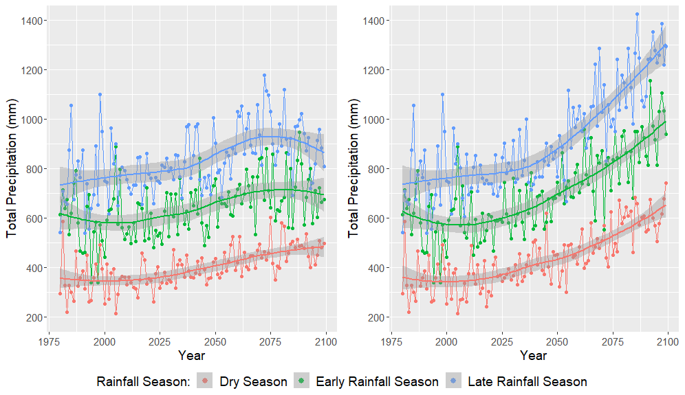
Figure 14CanESM2 average total precipitation (mm) per weather station by rainfall season for the RCP4.5 forcing scenario (left) and the RCP8.5 forcing scenario (right). The years 1980–2005 represent historical GHCN observations and are also included on these plots. The years 2006–2100 represent downscaled CanESM2 output. This figure was created using Wickham (2016).

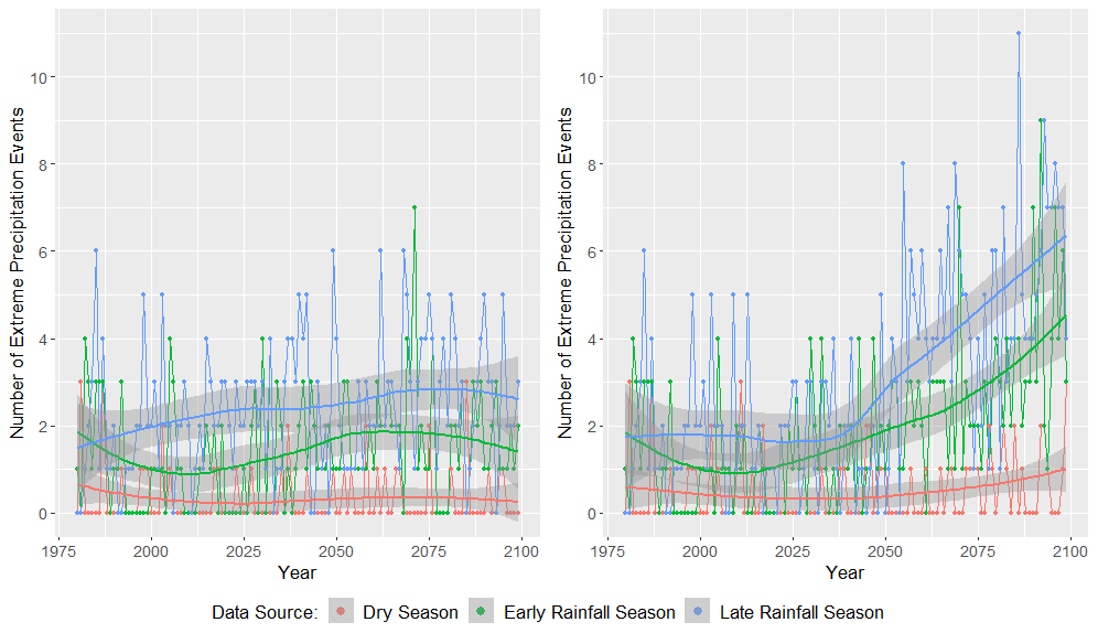
Figure 15Total number of extreme rainfall (ER) events (island daily average rainfall >29.90 mm) by season for the CanESM2's RCP4.5 forcing scenario (left) and the RCP8.5 forcing scenario (right). The years 1980–2005 represent historical GHCN observations and are also included on these plots. This figure was created using Wickham (2016).
In Fig. 14, we plot average total precipitation (in mm) across the 23 weather stations as a function of year and rainfall season. The RCP4.5 forcing scenario is plotted in the left panel, while the RCP8.5 forcing scenario is plotted in the right panel. Clearly, precipitation varies seasonally in Puerto Rico, where the dry season (December through March) tends to see the least rainfall, and the late rainfall season (August through November) tends to observe the most rainfall. The CanESM2 projections indicate that Puerto Rico's total precipitation will increase across each season for both the RCP4.5 and RCP8.5 forcing scenarios. However, the precipitation increases are much more dramatic under the latter. It is important to keep in mind that increased water demand from higher temperatures may more than offset any increased precipitation. In other words, it can still be “drier”, even with more rainfall.
Now, we explore the frequency of large-scale rainfall events. First, we define two types of high-magnitude rainfall events:
-
extreme rainfall (ER) events, any day such that the island daily average precipitation is larger than the 99th percentile of observed average daily precipitation totals from 1980 to 2005: 29.90 mm, and
-
high-magnitude rainfall (HMR) events, any day such that the island daily average precipitation is larger than the 95th percentile of observed average daily precipitation totals from 1980 to 2005: 14.81 mm.
Figure 15 displays the number of ER events as a function of rainfall season and year. The RCP4.5 emission scenario is displayed on the left, while the RCP8.5 emission scenario is displayed on the right. The RCP4.5 emission scenario indicates slight increases in ER events during the LRS and ERS. The RCP8.5 emission scenario indicates a substantial increase in the number of extreme rainfall events during the LRS and ERS. Under the RCP8.5 emission scenario, the LRS, or hurricane season, is projected to observe more than seven ER events each year, and the ERS is expected to see between four and five ER events each year, while the dry season (DS) is expected to continue to observe very few ER events by 2100.
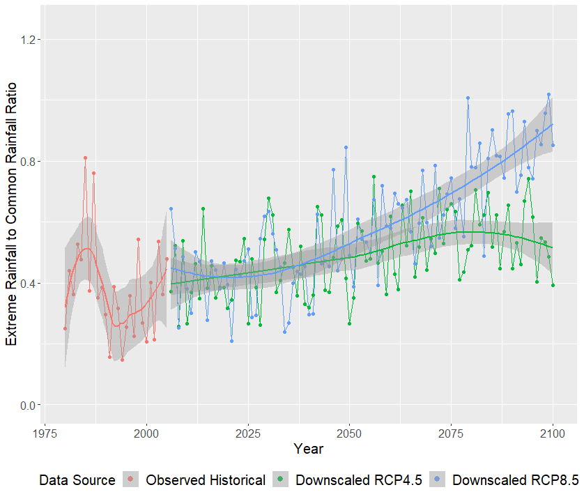
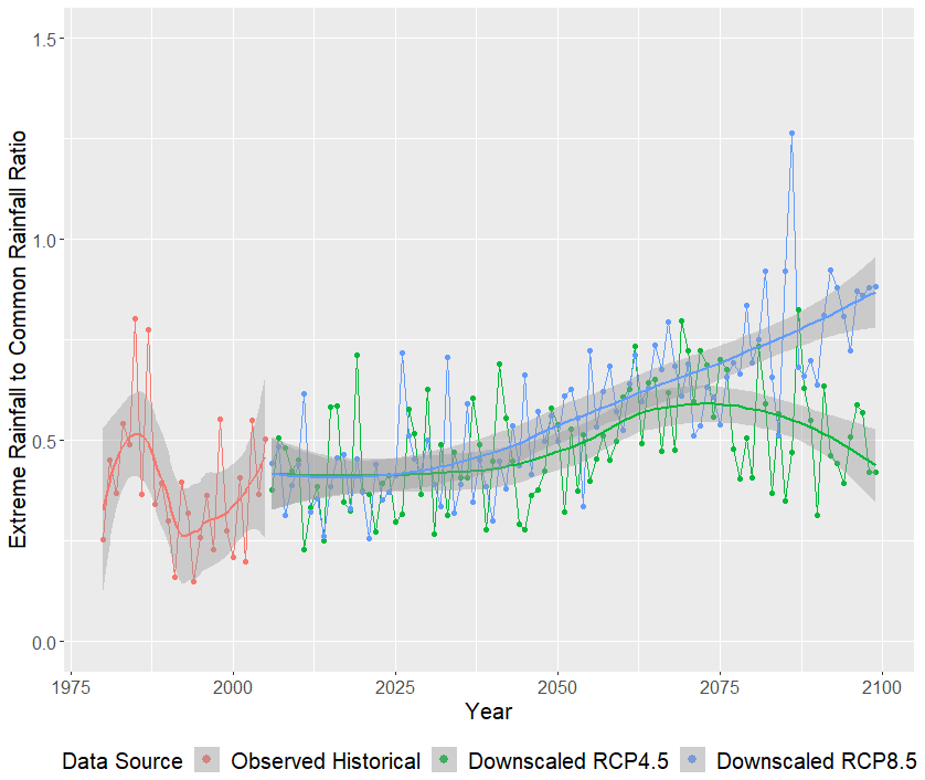
Figure 16 displays the ratio of yearly HMR event (island daily average >14.81 mm) total rainfall to the annual total of smaller rainfall events (island daily average ≤14.81 mm). Historically, the total rainfall from HMR events represented around 40 % of the total rainfall from more common precipitation events. The RCP4.5 emission scenario does not exhibit a clear shift in this relationship. However, in the RCP8.5 emission scenario, the proportion of yearly rainfall due to HMR events is projected to increase dramatically. By 2100, the ratio of yearly HMR to yearly rainfall more common events is nearly 1 : 1.
5.2 Summary of downscaled climate data
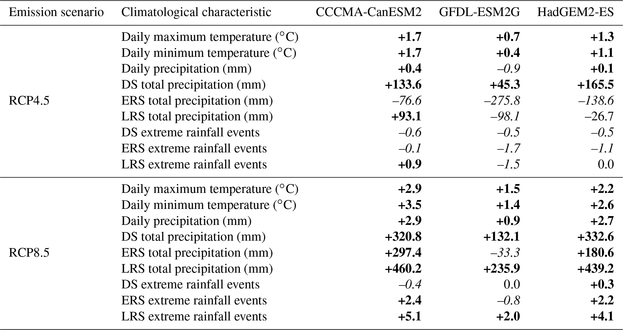
In Table 5, we display the approximate changes of several climatological characteristics from 2005 to 2100. Bolded and italicized cells are used to indicate increases and decreases of the specified feature. Approximate changes are calculated by first fitting separate LOESS smoothing splines to the historical and future data. We then take the difference between the LOESS estimates in 2100 and 2005. For the climate models and methods examined in this study, the RCP8.5 forcing scenario favors a dramatic increase in rainfall for Puerto Rico. The RCP4.5 forcing scenario favors much smaller increases in rainfall and even a noticeable decreases across the ERS. NOAA's GFDL under the RCP4.5 forcing scenario more closely matches projected rainfall patterns across the Caribbean from other studies (Biasutti et al., 2012; Cashman et al., 2010; Girvetz et al., 2009; Meehl et al., 2009).
Table 5Approximate changes of several climatological characteristics from 2005 to 2100. Bolded cells and italicized cells indicate increases and decreases of the specified feature.
In this work, we utilize a novel combination of downscaling methods of Jeong et al. (2012a, b). We employ a two-part multivariate multisite statistical downscaling model (MMSDM) to downscale maximum and minimum temperatures and precipitation at K=23 weather stations in Puerto Rico. To downscale precipitation, we first decompose it into two components: precipitation probability and log-transformed precipitation amount.
The MMSDM methodology is unable to correct GCM bias adequately. To quantify and correct for these biases, we propose LOESS quantile mapping (LQM), which combines elements of localized regression and quantile mapping. LQM employs standard quantile mapping techniques as a function of season, which we defined as Julian day. First, percentiles of observed and fitted values of a specified random variable are estimated as a function of season. Next, bias is estimated as a function of percentile and season by simply taking the difference between the observed and fitted summaries. Then, LOESS smoothing techniques are applied to the bias values, and the bias is estimated via LOESS regression as a function of season. Finally, the estimated bias, which is allowed to vary as a function of percentile (as in standard quantile mapping) and season (the extension to standard QM), is added directly to the fitted values (and subsequently added directly to the downscaled climate projections).
We proceed to combine these new extensions in order to study the future climate of Puerto Rico. The resulting downscaled temperature projections from the three climate models all agree that Puerto Rico will experience a warmer future climate. These projections are consistent with the overwhelming majority of published literature examining future Caribbean climate (Biasutti et al., 2012; Jennings et al., 2014). Not only will Puerto Rico experience a warmer climate, but the average day will also have a narrower temperature range as minimum temperatures are expected to increase at a faster rate than maximum temperatures. The RCP8.5 forcing scenario (carbon emissions continue to grow through the year 2100) projects a warmer climate than that of the RCP4.5 forcing scenario (carbon emissions are curbed and do not grow after a certain date). The majority of literature agrees that the Caribbean will see reduced rainfall in its future climate (Bowden et al., 2021; He and Soden, 2017). Within the RCP4.5 forcing scenario, our methods tend to be consistent with those of the literature. The three models explored here agree that the DS will observe increased rainfall, while the ERS and LRS will likely observe a decline in total rainfall. However, GCM output from the RCP8.5 forcing scenario tends to favor the opposite: a wetter climate for Puerto Rico, driven by an increase in extreme rainfall events.
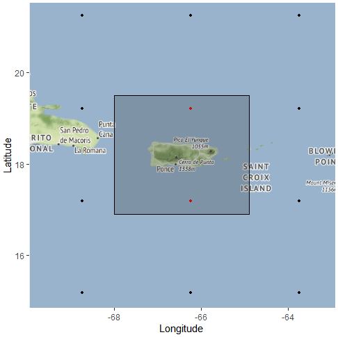
Figure A1The bounding box for which GCM coordinates are kept (latitudes range from 16.90 to 19.50∘, and longitudes range from −68.00 to −64.90∘). ESM2G locations inside the box (red) are kept, while ESM2G locations outside the box (black) are not kept. Note that the bounding box was only extended for this model. This image was created using a combination of © Google Maps 2018, Kahle and Wickham (2013), and Wickham (2016).
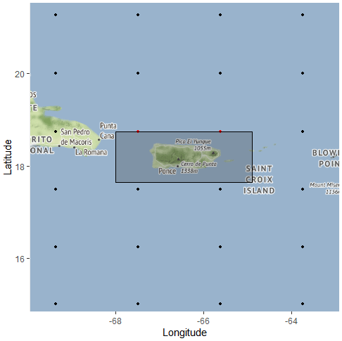
Figure A2The bounding box for which GCM coordinates are kept (latitudes range from 17.65 to 18.75∘, and longitudes range from −68.00 to −64.90∘). HadGEM2-ES locations inside the box (red) are kept, while HadGEM2-ES locations outside the box (black) are not kept. This image was created using a combination of © Google Maps 2018, Kahle and Wickham (2013), and Wickham (2016).
B1 Temperature
Table B1ESM2G maximum daily temperature quantiles (∘C, top panel) and minimum daily temperature quantiles (∘C, bottom panel) for the observed historical (from GHCN) climate, the downscaled RCP4.5 climate, and the downscaled RCP8.5 climate.
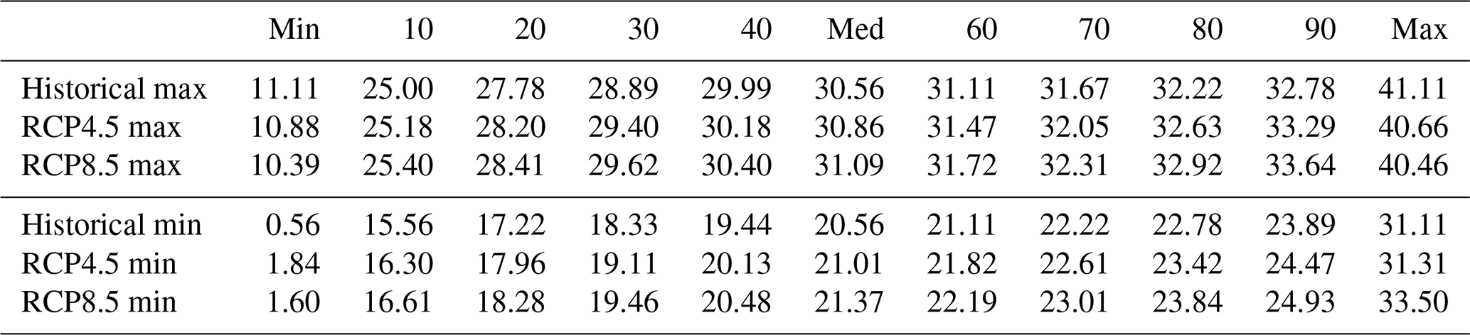
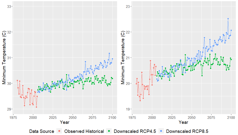
Figure B1ESM2G mean daily maximum (left panel) and minimum (right panel) temperature (∘C) as a function of year. Observed historical GHCN data from 1980–2005 are plotted in red, while downscaled RCP4.5 and RCP8.5 temperatures from 2006–2100 are plotted in green and blue, respectively. This figure was created using Wickham (2016).
B2 Precipitation
Table B2ESM2G daily total precipitation (mm) quantiles for the observed historical GHCN climate, the downscaled RCP4.5 climate, and the downscaled RCP8.5 climate.


C1 Temperature
Table C1Maximum daily temperature quantiles (∘C, top panel) and minimum daily temperature quantiles (∘C, bottom panel) for the observed historical GHCN climate, the downscaled RCP4.5 climate, and the downscaled RCP8.5 climate using the Hadley Centre's HadGEM2-ES.

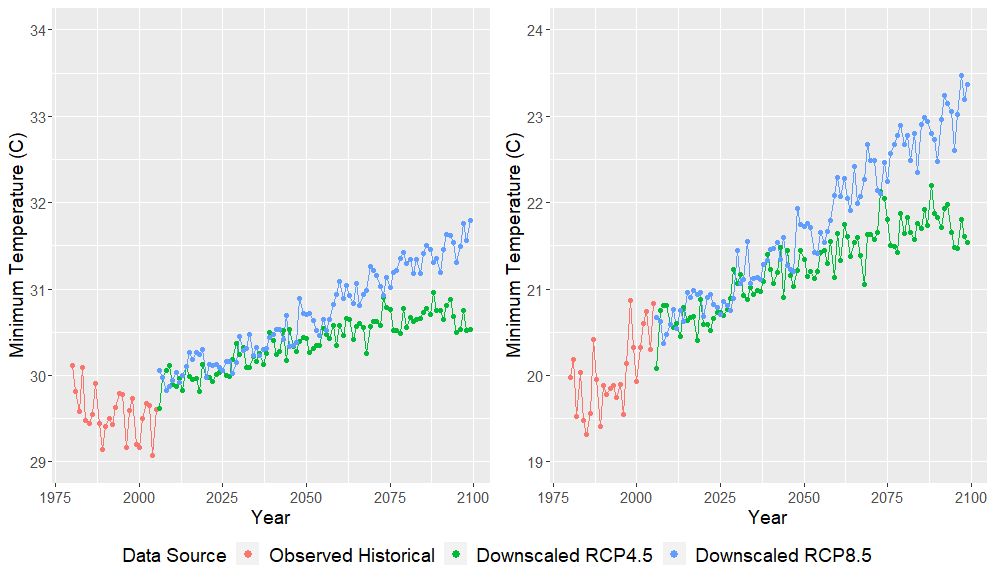
Figure C1Mean daily maximum (left panel) and minimum (right panel) temperature (∘C) as a function of year. Observed historical GHCN data from 1980–2005 are plotted in red, while downscaled RCP4.5 and RCP8.5 temperatures (from the UK's HadGEM2) from 2006–2100 are plotted in green and blue, respectively. This figure was created using Wickham (2016).
C2 Precipitation
Table C2Daily total precipitation (mm) quantiles for the observed historical GHCN climate, the downscaled RCP4.5 climate, and the downscaled RCP8.5 climate using the UK's HadGEM2-ES.

R codes for performing the statistical analyses described in this paper are available at https://github.com/captseymour/MMSDM (last access: 31 December 2022). The most up-to-date published code is available on Zenodo at https://doi.org/10.5281/zenodo.7497210 (Washington and Seymour, 2022).
All data used in this study are publicly available. The primary historical climate data are from the publicly available Global Historical Climatological Network (GHCN; Menne et al., 2012a, b). The CMIP5 GCM data were downloaded using the Department of Energy Lawrence Livermore National Laboratory's (DOE/LLNL) data retrieval tool (https://esgf-node.llnl.gov/search/cmip5/, DOE/LLNL, 2023).
This work, including the code, was originally completed as part of Benjamin Washington's doctoral dissertation in statistics, under the direction of Lynne Seymour. Thomas Mote provided the necessary expertise on the climate modeling, especially as it pertains to Puerto Rico.
The contact author has declared that none of the authors has any competing interests.
Publisher’s note: Copernicus Publications remains neutral with regard to jurisdictional claims in published maps and institutional affiliations.
Support for Thomas Mote was provided by the National Science Foundation's (NSF's) Long Term Ecological Research (LTER) grant. We are appreciative of climate data efforts such as the GHCN, which is maintained by the National Oceanic and Atmospheric Administration's (NOAA's) National Centers for Environmental Information (NCEI, 2018). Additionally, we are grateful to GCM climate projects such as CMIP. CMIP5 GCM data are made publicly available via the Department of Energy Lawrence Livermore National Laboratory's (DOE/LLNL) data retrieval tool. GCM data would not be publicly available without the support of the Earth System Grid Federation (ESGF), whose aim is to enhance software that powers most GCMs (Ananthakrishnan et al., 2013; Cinquini et al., 2014). Thanks to the ESGF, multiple petabytes of GCM data are publicly available online on many federal websites, the LLNL being one of them.
This research has been supported by National Science Foundation Luquillo Long-Term Ecological Research Program (grant no. DEB1239764).
This paper was edited by Michael Wehner and reviewed by Adam Terando and one anonymous referee.
Ananthakrishnan, R., Bell, G., Cinquini, L., Crichton, D., Danvil, S., Drach, B., Fiore, S., Gonzalez, E., Harney, J. F., and Mattmann, C.: The Earth System Grid Federation: An Open Infrastructure for Access to Distributed Geospatial Data, Tech. rep., Oak Ridge National Lab.(ORNL), Oak Ridge, TN (United States), Center for Computational Sciences, https://doi.org/10.1016/j.future.2013.07.002, 2013. a
Angeles, M. E., Gonzalez, J. E., Erickson III, D. J., and Hernández, J. L.: Predictions of future climate change in the Caribbean region using global general circulation models, Int. J. Climatol., 27, 555–569, 2007. a
Angeles, M. E., González, J. E., Ramírez-Beltrán, N. D., Tepley, C. A., and Comarazamy, D. E.: Origins of the Caribbean rainfall bimodal behavior, J. Geophys. Res.-Atmos., 115, D11106, https://doi.org/10.1029/2009JD012990, 2010. a, b
Ben Alaya, M. A., Chebana, F., and Ouarda, T.: Probabilistic Gaussian copula regression model for multisite and multivariable downscaling, J. Climate, 27, 3331–3347, 2014. a
Bhardwaj, A., Misra, V., Mishra, A., Wootten, A., Boyles, R., Bowden, J., and Terando, A. J.: Downscaling future climate change projections over Puerto Rico using a non-hydrostatic atmospheric model, Climatic Change, 147, 133–147, 2018. a
Biasutti, M., Sobel, A. H., Camargo, S. J., and Creyts, T. T.: Projected changes in the physical climate of the Gulf Coast and Caribbean, Climatic Change, 112, 819–845, 2012. a, b, c, d, e, f
Bowden, J. H., Terando, A. J., Misra, V., Wootten, A., Bhardwaj, A., Boyles, R., Gould, W., Collazo, J. A., and Spero, T. L.: High-resolution dynamically downscaled rainfall and temperature projections for ecological life zones within Puerto Rico and for the US Virgin Islands, Int. J. Climatol., 41, 1305–1327, 2021. a, b, c
Campbell, J. D., Taylor, M. A., Stephenson, T. S., Watson, R. A., and Whyte, F. S.: Future climate of the Caribbean from a regional climate model, Int. J. Climatol., 31, 1866–1878, 2011. a, b, c
Cannon, A. J.: Multivariate quantile mapping bias correction: an N-dimensional probability density function transform for climate model simulations of multiple variables, Clim. Dynam., 50, 31–49, 2018. a, b, c
Cashman, A., Nurse, L., and John, C.: Climate change in the Caribbean: The water management implications, J. Environ. Dev., 19, 42–67, 2010. a, b
Centella, A., Bezanilla, A., and Leslie, K.: Technical report: A study of the uncertainty in future Caribbean climate using the PRECIS regional climate model, Institute of Meteorology, Community Caribbean Climate Change Centre, Cuba, https://www.eldis.org/document/A60777 (last access: 26 January 2023), 2008. a
Chen, A. A. and Taylor, M. A.: Investigating the link between early season Caribbean rainfall and the El Niño+ 1 year, Int. J. Climatol., 22, 87–106, 2002. a
Chen, D., Dai, A., and Hall, A.: The Convective-To-Total Precipitation Ratio and the “Drizzling” Bias in Climate Models, J. Geophys. Res.-Atmos., 126, e2020JD034198, https://doi.org/10.1029/2020JD034198, 2021. a
Cinquini, L., Crichton, D., Mattmann, C., Harney, J., Shipman, G., Wang, F., Ananthakrishnan, R., Miller, N., Denvil, S., and Morgan, M.: The Earth System Grid Federation: An open infrastructure for access to distributed geospatial data, Future Gener. Comp. Sy., 36, 400–417, 2014. a
Cleveland, W. S., Grosse, E., and Shyu, W. M.: Local regression models, in: Statistical Models in S, Routledge, 309–376, ISBN 9780203738535, 2017. a, b
Comarazamy, D. E. and González, J. E.: On the validation of the simulation of early season precipitation on the island of Puerto Rico using a mesoscale atmospheric model, J. Hydrometeorol., 9, 507–520, 2008. a
Department of Energy Lawrence Livermore National Laboratory (DOE/LLNL): World Climate Research Programme CMIP5, https://esgf-node.llnl.gov/search/cmip5, last access: 26 January 2023. a
Girvetz, E. H., Zganjar, C., Raber, G. T., Maurer, E. P., Kareiva, P., and Lawler, J. J.: Applied climate-change analysis: the climate wizard tool, PLoS One, 4, https://doi.org/10.1371/journal.pone.0008320, 2009. a, b
Guo, Q., Chen, J., Zhang, X., Shen, M., Chen, H., and Guo, S.: A new two-stage multivariate quantile mapping method for bias correcting climate model outputs, Clim. Dynam., 53, 3603–3623, 2019. a
Gutowski Jr., W. J., Decker, S. G., Donavon, R. A., Pan, Z., Arritt, R. W., and Takle, E. S.: Temporal-spatial scales of observed and simulated precipitation in central US climate, J. Climate, 16, 3841–3847, 2003. a
Harmsen, E. W., Miller, N. L., Schlegel, N. J., and Gonzalez, J. E.: Seasonal climate change impacts on evapotranspiration, precipitation deficit and crop yield in Puerto Rico, Agr. Water Manage., 96, 1085–1095, 2009. a
He, J. and Soden, B. J.: A re-examination of the projected subtropical precipitation decline, Nat. Clim. Change, 7, 53–57, 2017. a, b
Jennings, L. N., Douglas, J., Treasure, E., and González, G.: Climate change effects in El Yunque National Forest, Puerto Rico, and the Caribbean region, General Technical Report SRS-GTR-193, Asheville, NC, USDA-Forest Service, Southern Research Station, 193, 1–47, https://doi.org/10.2737/SRS-GTR-193, 2014. a, b
Jeong, D. I., St-Hilaire, A., Ouarda, T., and Gachon, P.: A multivariate multi-site statistical downscaling model for daily maximum and minimum temperatures, Clim. Res., 54, 129–148, 2012a. a, b, c, d
Jeong, D. I., St-Hilaire, A., Ouarda, T. B., and Gachon, P.: Multisite statistical downscaling model for daily precipitation combined by multivariate multiple linear regression and stochastic weather generator, Climatic Change, 114, 567–591, 2012b. a, b, c
Kahle, D. and Wickham, H.: ggmap: Spatial Visualization with ggplot2, R J., 5, 144–161, 2013. a, b, c, d
Khalyani, A. H., Gould, W. A., Harmsen, E., Terando, A., Quinones, M., and Collazo, J. A.: Climate change implications for tropical islands: Interpolating and interpreting statistically downscaled GCM projections for management and planning, J. Appl. Meteorol. Clim., 55, 265–282, 2016. a
Lafon, T., Dadson, S., Buys, G., and Prudhomme, C.: Bias correction of daily precipitation simulated by a regional climate model: a comparison of methods, Int. J. Climatol., 33, 1367–1381, 2013. a
Lashof, D. A. and Ahuja, D. R.: Relative contributions of greenhouse gas emissions to global warming, Nature, 344, 529–531, 1990. a
Lintner, B. R., Biasutti, M., Diffenbaugh, N. S., Lee, J.-E., Niznik, M. J., and Findell, K. L.: Amplification of wet and dry month occurrence over tropical land regions in response to global warming, J. Geophys. Res.-Atmos., 117, D11106, https://doi.org/10.1029/2012JD017499, 2012. a
Lund, R., Hurd, H., Bloomfield, P., and Smith, R.: Climatological time series with periodic correlation, J. Climate, 8, 2787–2809, 1995. a
Magrin, G., Gay Garcia, C., Cruz Choque, D., Gimenez-Sal, J., Moreno, A., Nagy, G., Nobre, C., and Villamizar, A.: Climate Change and Climate Variability in the Latin American Region, in: American Geophysical Union Spring Meeting Abstracts, https://ui.adsabs.harvard.edu/abs/2007AGUSM.U33B..02M (last access: 23 January 2023), 2007. a, b
Maraun, D.: Bias correction, quantile mapping, and downscaling: Revisiting the inflation issue, J. Climate, 26, 2137–2143, 2013. a
Maraun, D.: Bias correcting climate change simulations – A critical review, Current Climate Change Reports, 2, 211–220, 2016. a
Mattingly, K. S., Seymour, L., and Miller, P. W.: Estimates of Extreme Precipitation Frequency Derived from Spatially Dense Rain Gauge Observations: A Case Study of Two Urban Areas in the Colorado Front Range Region, Ann. Am. Assoc. Geogr., 107, 1499–1518, 2017. a
Meehl, G. A., Covey, C., Delworth, T., Latif, M., McAvaney, B., Mitchell, J. F., Stouffer, R. J., and Taylor, K. E.: The WCRP CMIP3 multimodel dataset: A new era in climate change research, B. Am. Meteorol. Soc., 88, 1383–1394, 2007. a
Meehl, G. A., Goddard, L., Murphy, J., Stouffer, R. J., Boer, G., Danabasoglu, G., Dixon, K., Giorgetta, M. A., Greene, A. M., and Hawkins, E. D.: Decadal prediction: can it be skillful?, B. Am. Meteorol. Soc., 90, 1467–1486, 2009. a
Meinshausen, M., Meinshausen, N., Hare, W., Raper, S. C., Frieler, K., Knutti, R., Frame, D. J., and Allen, M. R.: Greenhouse-gas emission targets for limiting global warming to 2 ∘C, Nature, 458, 1158–1162, 2009. a
Menne, M. J., Durre, I., Korzeniewski, B., McNeill, S., Thomas, K., Yin, X., Anthony, S., Ray, R., Vose, R. S., Gleason, B. E., and Houston, T. G.: Global Historical Climatology Network – Daily (GHCN-Daily), Version 3. [Puerto Rico], NOAA National Climatic Data Center [data set], https://doi.org/10.7289/V5D21VHZ, 2012a. a
Menne, M. J., Durre, I., Vose, R. S., Gleason, B. E., and Houston, T. G.: An Overview of the Global Historical Climatology Network-Daily Database, J. Atmos. Ocean. Tech., 29, 897–910, https://doi.org/10.1175/JTECH-D-11-00103.1, 2012b. a
Miller, P. W., Mote, T. L., and Ramseyer, C. A.: An Empirical Study of the Relationship between Seasonal Precipitation and Thermodynamic Environment in Puerto Rico, Weather Forecast., 34, 277–288, 2019. a
Müller, C., Cramer, W., Hare, W. L., and Lotze-Campen, H.: Climate change risks for African agriculture, P. Natl. Acad. Sci. USA, 108, 4313–4315, https://doi.org/10.1073/pnas.1015078108, 2011. a
NCEI: National Centers for Environmental Information's Daily Observational Data Map, Version 2.2.0, https://gis.ncdc.noaa.gov/maps/ncei/cdo/daily, last access: 1 December 2018. a
Nesbitt, S. W., Cifelli, R., and Rutledge, S. A.: Storm morphology and rainfall characteristics of TRMM precipitation features, Mon. Weather Rev., 134, 2702–2721, 2006. a
Park, J., Kang, M. S., and Song, I.: Bias correction of RCP-based future extreme precipitation using a quantile mapping method; for 20-weather stations of South Korea, Journal of the Korean Society of Agricultural Engineers, 54, 133–142, 2012. a
Pierce, D. W., Cayan, D. R., and Thrasher, B. L.: Statistical downscaling using localized constructed analogs (LOCA), J. Hydrometeorol., 15, 2558–2585, 2014. a
Ramirez-Villegas, J., Challinor, A. J., Thornton, P. K., and Jarvis, A.: Implications of regional improvement in global climate models for agricultural impact research, Environ. Res. Lett., 8, 024018, https://doi.org/10.1088/1748-9326/8/2/024018, 2013. a
Ramseyer, C., Miller, P., and Mote, T. L.: Statistical Downscaling of CMIP5 data to predict future dry day frequency in the El Yunque National Forest, in: American Geophysical Union Fall Meeting Abstracts, vol. 2018, A21L–2904, https://ui.adsabs.harvard.edu/abs/2018AGUFM.A21L2904R (last access: 23 January 2023), 2018. a, b
Ramseyer, C. A. and Mote, T. L.: Atmospheric controls on Puerto Rico precipitation using artificial neural networks, Clim. Dynam., 47, 2515–2526, 2016. a, b
Ramseyer, C. A. and Mote, T. L.: Analysing regional climate forcing on historical precipitation variability in Northeast Puerto Rico, Int. J. Climatol., 38, e224–e236, 2018. a, b
Ramseyer, C. A., Miller, P. W., and Mote, T. L.: Future precipitation variability during the early rainfall season in the El Yunque National Forest, Sci. Total Environ., 661, 326–336, 2019. a, b
Satterthwaite, D.: Cities' contribution to global warming: notes on the allocation of greenhouse gas emissions, Environ. Urban., 20, 539–549, 2008. a
Stennett-Brown, R. K., Jones, J. J., Stephenson, T. S., and Taylor, M. A.: Future Caribbean temperature and rainfall extremes from statistical downscaling, Int. J. Climatol., 37, 4828–4845, 2017. a
Taylor, K. E., Balaji, V., Hankin, S., Juckes, M., Lawrence, B., and Pascoe, S.: CMIP5 Data Reference Syntax (DRS) and Controlled Vocabularies, in: Program for Climate Model Diagnosis and Intercomparison, http://pcmdi.github.io/mips/cmip5/docs/cmip5_data_reference_syntax.pdf (last access: 23 January 2023), 2011. a, b
Taylor, K. E., Stouffer, R. J., and Meehl, G. A.: An overview of CMIP5 and the experiment design, B. Am. Meteorol. Soc., 93, 485–498, 2012. a
Taylor, M. A., Enfield, D. B., and Chen, A. A.: Influence of the tropical Atlantic versus the tropical Pacific on Caribbean rainfall, J. Geophys. Res.-Oceans, 107, 3127, https://doi.org/10.1029/2001JC001097, 2002. a, b
Thrasher, B., Maurer, E. P., McKellar, C., and Duffy, P. B.: Technical Note: Bias correcting climate model simulated daily temperature extremes with quantile mapping, Hydrol. Earth Syst. Sci., 16, 3309–3314, https://doi.org/10.5194/hess-16-3309-2012, 2012. a, b, c, d
Van Beusekom, A. E., Gould, W. A., Terando, A. J., and Collazo, J. A.: Climate change and water resources in a tropical island system: propagation of uncertainty from statistically downscaled climate models to hydrologic models, Int. J. Climatol., 36, 3370–3383, 2016. a
Washington, B. and Seymour, L.: An Adapted vector Autoregressive Expectation-Maximization Imputation Algorithm for Climate Data Networks, Wires Comput. Stat., 12, e1494, https://doi.org/10.1002/wics.1494, 2019. a
Washington, B., Seymour, L., Lund, R., and Willett, K.: Simulation of temperature series and small networks from data, Int. J. Climatol., 39, 5104–5123, 2019. a, b
Washington, B. J. and Seymour, L.: captseymour/MMSDM: Code for Washington, Seymour, and Mote (2023), Zenodo [code], https://doi.org/10.5281/zenodo.7497210, 2022. a
Wickham, H.: ggplot2: Elegant Graphics for Data Analysis, Springer-Verlag New York, http://ggplot2.org (last access: 22 January 2023), 2016. a, b, c, d, e, f, g, h, i, j, k, l, m, n, o, p, q, r, s, t, u, v, w, x, y, z, aa, ab
Winkler, J. A., Palutikof, J. P., Andresen, J. A., and Goodess, C. M.: The simulation of daily temperature time series from GCM output. Part II: Sensitivity analysis of an empirical transfer function methodology, J. Climate, 10, 2514–2532, 1997. a
Wood, A. W., Maurer, E. P., Kumar, A., and Lettenmaier, D. P.: Long-range experimental hydrologic forecasting for the eastern United States, J. Geophys. Res.-Atmos., 107, 4429, https://doi.org/10.1029/2001JD000659, 2002. a, b
Yang, C., Chandler, R. E., Isham, V. S., and Wheater, H. S.: Spatial-temporal rainfall simulation using generalized linear models, Water Resour. Res., 41, W11415, https://doi.org/10.1029/2004WR003739, 2005. a
- Abstract
- Introduction
- Data sources and cleaning
- Spatial downscaling methodology
- Bias-correction methods
- Puerto Rico downscaled climate projections
- Summary
- Appendix A: GCM climate plots
- Appendix B: USA GFDL's ESM2G downscaled climate
- Appendix C: UK's HadGEM2-ES downscaled climate
- Code availability
- Data availability
- Author contributions
- Competing interests
- Disclaimer
- Acknowledgements
- Financial support
- Review statement
- References