the Creative Commons Attribution 4.0 License.
the Creative Commons Attribution 4.0 License.
 | 14 Jul 2023
Quantifying the statistical dependence of mid-latitude heatwave intensity and likelihood on prevalent physical drivers and climate change
Erich M. Fischer
Recent heatwaves such as the 2021 Pacific Northwest heatwave have shattered temperature records across the globe. The likelihood of experiencing extreme temperature events today is already strongly increased by anthropogenic climate change, but it remains challenging to determine to what degree prevalent atmospheric and land surface conditions aggravated the intensity of a specific heatwave event. Quantifying the respective contributions is therefore paramount for process understanding but also for attribution and future projection statements conditional on the state of atmospheric circulation or land surface conditions. We here propose and evaluate a statistical framework based on extreme value theory, which enables us to learn the respective statistical relationship between extreme temperature and process variables in initial-condition large ensemble climate model simulations. Elements of statistical learning theory are implemented in order to integrate the effect of the governing regional circulation pattern. The learned statistical models can be applied to reanalysis data to quantify the relevance of physical process variables in observed heatwave events. The method also allows us to make conditional attribution statements and answer “what if” questions. For instance, how much would a heatwave intensify given the same dynamic conditions but at a different warming level? How much additional warming is needed for the same heatwave intensity to occur under average circulation conditions? Changes in the exceedance probability under varying large- and regional-scale conditions can also be assessed. We show that each additional degree of global warming increases the 7 d maximum temperature for the Pacific Northwest area by almost 2 ∘C, and likewise, we quantify the direct effect of anti-cyclonic conditions on heatwave intensity. Based on this, we find that the combined global warming and circulation effect of at least 2.9 ∘C accounts for 60 %–80 % of the 2021 excess event intensity relative to average pre-industrial heatwave conditions.
- Article
(5790 KB) - Full-text XML
-
Supplement
(22838 KB) - BibTeX
- EndNote


Heatwave events pose a substantial risk to ecosystems (Stillman, 2019) and the economy (Jahn, 2015), but specifically to human health and wellbeing (Vicedo-Cabrera et al., 2021), especially in combination with compound perils: increased air pollution (Fischer et al., 2004; Shaposhnikov et al., 2014) or fire risk (Parente et al., 2018; Deb et al., 2020) and heat-drought-induced crop failure (Ribeiro et al., 2020; Beillouin et al., 2020). The adverse effects of temperature extremes, which are especially destructive for developing countries (Akhtar, 2020), should be expected to worsen as anthropogenic climate change affects hot extremes almost globally today already (IPCC, 2021). In the past decades, several heatwave events of unprecedented intensity, many exceeding previous records by large margins (Barriopedro et al., 2011; Fischer et al., 2021), stimulated public interest and initiated academic efforts in extreme event attribution (Stott et al., 2004). For the latter, isolating anthropogenic effects from natural effects is necessary. By also quantifying the contributions of thermodynamic and dynamic drivers, the mechanistic understanding, attribution and future projection of heatwave events can be further improved (Vautard et al., 2016).
1.1 Research objective
The objective of this study is to disentangle the effects of different physical drivers on low-likelihood heatwave events. It should provide estimates of how much prevalent dynamic and thermodynamic configurations contributed to the intensity of observed extreme heat events but also allow “what if” questions to be answered, for example how much the intensity of a specific event would be altered under different climatic conditions. The focus on low-likelihood heat extremes and the limited availability of observational data require one to learn the statistical relationships of heat extreme intensity and selected covariates from simulated heatwave data, which are provided in single-model initial-condition large ensemble climate simulations. The primary dataset used in this study is an 84-member large ensemble of the Community Earth System Model version 1.2 (CESM12), and non-stationary extreme value modelling provides the methodological framework for the analysis. The main focus is on the Pacific Northwest (PNW) area, but statistical models are also retrieved for western Europe (WEU) and western Russia (WRU), where well-studied record-breaking heat extremes occurred in the past decades (area-of-interest definitions are provided in Supplement Table S2).
The intensity of extreme heatwave events at the mid-latitudes is determined by a multitude of climatological factors across various spatio-temporal scales (Perkins, 2015; Horton et al., 2016; Domeisen et al., 2022). For the purposes of this study, we identify the three primary classes of (1) global thermodynamic, (2) local land surface and (3) regional tropospheric circulation conditions relevant for mid-latitude heat extremes, acknowledging the fact that an objective separation into distinct categories is hardly possible given the coupled nature of the climate system. Global-scale and multi-decadal thermodynamic temperature trends and decadal regional temperature variability driven by ocean circulation or sea ice variability govern the long-term conditions affecting heatwave intensity (Schär et al., 2004; Della-Marta et al., 2007b; Fischer and Schär, 2009; Feudale and Shukla, 2011; Kröner et al., 2017). Local, short-term (weekly to seasonal) land surface conditions like soil moisture or snow cover determine the surface energy budget prior to and during the build-up of a heat extreme (Fischer et al., 2007; Vogel et al., 2017). Finally, the necessary clear-sky conditions (diabatic warming), subsidence (adiabatic warming) and advection of warm air are determined by regional, short-term (days to weeks) and anti-cyclonic circulation conditions (Rex, 1950; Pfahl and Wernli, 2012; Horton et al., 2015; Bieli et al., 2015).
Representing both dynamic and thermodynamic processes across the spectrum of spatio-temporal scales in the same model is required to accurately explain the intensity of heat extremes (Della-Marta et al., 2007b) and to avoid overestimating the independent statistical effect of a single process variable (Suarez-Gutierrez et al., 2020). The selection of relevant process variables is further affected by the following constraints: the variables should have a (close-to) unidirectional causal relationship with heatwave intensity, with little potential for feedback effects, to avoid artefacts due to phenomena like the “heat low” in surface pressure (Rácz and Smith, 1999) or the temperature dependence of the evaporative fraction. Furthermore, the separation of effects requires minimal inter-dependency between process variables, avoiding statistical artefacts of collinearity. Finally, the respective data must be available and comparable amongst various climate model and observational or reanalysis datasets. Taking these criteria into account, the following process variables are selected as statistical predictors.
-
Smoothed global mean surface temperature (GMST) as a proxy for long-term climatic changes and the respective thermodynamic forcing of local heat extremes
-
Soil moisture (SM) as a proxy for local land surface and soil conditions
-
Geopotential height of the 500 hPa pressure surface (Z500) as a proxy for the regional circulation field. By including not just the local (grid-point-average) geopotential height anomaly, but also the regional field, we aim at also representing non-local dynamical effects, such as advection, on heat extremes.
It is evident that the issue of collinearity has to be addressed, since trends in both SM and Z500 are clearly driven by long-term climatic change. Furthermore, differences in variables across datasets (absolute values and variability) have to be accounted for. Thus, the pre-processing of these variables entails the removal of a climate change signal and a dataset-specific standardisation. Given the importance of the underlying data quality and pre-processing, the respective evaluation and processing steps are outlined in Sect. 2. Section 3 introduces the parameterisation and the strategy to evaluate the merit of the statistical model. The estimated parameters, which quantitatively describe the linear relationship between process variables and heatwave intensity, are discussed in Sect. 4. The respective GEV models are then applied to PNW event data from ERA5 to study the effect sizes of the selected process variables. Section 4 also contains a discussion of the conditional PNW event intensity and likelihood changes under varying levels of global warming and the contributing circulation effect.
The statistical analysis of extreme climate events requires careful curation of data and application of methods, as results may depend heavily on seemingly negligible processing steps. The need for timely and robust extreme event attribution statements gave rise to a set of best-practice protocols, such as Ghil et al. (2011), Yiou et al. (2017), Philip et al. (2020), or Naveau et al. (2020). Many processing steps outlined in this and the following section are inspired by these protocols and contain specific elements thereof. This section provides background information on the data sources and outlines the pre-processing strategy. Detailed technical information is provided in Supplement Sect. S1.
2.1 Climate model and reanalysis datasets
For the training of the statistical model, we rely on Earth system model simulations, as only this data source provides the required number of extreme heatwave samples where the respective processes are represented at an adequate degree in past, present and future global climate states. The following analysis is primarily based on an exhaustive simulation set of the initial-condition large ensemble of CESM12, and additional simulations of the Coupled Model Intercomparison Project Phase 6 (CMIP6; Eyring et al., 2016) are also considered for validation purposes: see Table 1. These multiple single-model initial-condition large ensembles allow the implicit assessment of the uncertainty induced by internal climate variability (Deser et al., 2016; Lehner et al., 2020). Statistical models are estimated for each climate model dataset separately (i.e. there is no pooling of data across climate models) to fully characterise the inter-model uncertainty. These statistical models are later applied to past heatwave events in ERA5 and ERA5-Land reanalysis data (1950–2021) provided by the European Centre for Medium-Range Weather Forecasts (ECMWF) (Hersbach et al., 2020; Muñoz-Sabater et al., 2021).
Simulations of the CESM12 model (Hurrell et al., 2013) – consisting of and fully coupling the Community Atmosphere Model CAM version 5 (CAM5; Neale et al., 2012), the Community Land Model version 4 (CLM4; Lawrence et al., 2011), the Parallel Ocean Program version 2 (POP2; Smith et al., 2010) and further model components – constitute the primary basis of the training data. The simulations are comprised of a pre-industrial control simulation of 4780 years with constant forcing (not including an initial 500 year spin-up period to reach a steady-state equilibrium) and a total of 84 transient simulations; an ensemble of 21 members is initiated at various time points (and thus different oceanic states) of the pre-industrial control simulation, of which an additional three simulations per member are branched off in 1940 with a random perturbation of 10−14 K of the atmospheric temperature field. After 2006, these transient simulations follow the Representative Concentration Pathway (RCP)-8.5 forcing scenario until the end of the century. These data have been used for previous studies on the upper limit of heatwave intensity (Gessner et al., 2021) and the changing likelihood of heat extreme records (Fischer et al., 2021), as the respective processes are found to be adequately represented in the CESM1 climate model (see Supplement Sect. S1.1).
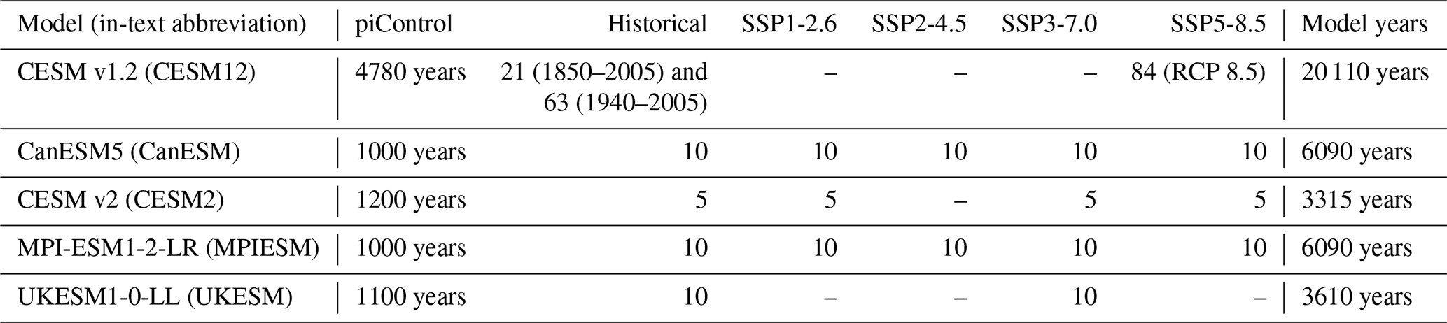
CMIP6 data were selected upon availability from the archive (Brunner et al., 2020), requiring at least 1000 years of pre-industrial simulations and at least 10 transient ensemble members with historical scenario forcings (1850–2014) and at least one tier-1 future (2015–2100) scenario forcing (Shared Socioeconomic Pathway (SSP) and end-of-century forcing combinations SSP1-2.6, SSP2-4.5, SSP3-7.0 and SSP5-8.5; O'Neill et al., 2016). Additionally, CESM version 2 (CESM2) data were included for the long pre-industrial control run (1200 years) and in order to compare results with the earlier model version CESM12. Furthermore, daily mean temperature and geopotential height data were required at daily and soil moisture data at monthly temporal resolution. An overview of the model–forcing combinations is provided in Table 1.
Table 1Length of the pre-industrial control run, the number of historical and transient future ensemble members per model and forcing scenario, and the resulting combined number of model years.
2.2 Data pre-processing
We here define the heatwave predictant variable as the 5-year maxima of 7 d running mean temperature (Tx7d), averaged over a spatial domain of interest (e.g. the PNW region shown in the yellow box in Fig. 2a). The 5-year block size is motivated by statistical considerations outlined in Sect. 3.2, and the 7 d averaging ensures that extreme events are analysed which persist for several days and are not just short-term temperature excursions. Tx7d data were not further pre-processed, in contrast to the physical process variables used as predictors.
In order to compare effect sizes and apply the statistical models to reanalysis data, the predictor variables should have comparable statistical metrics across datasets, i.e. a similar mean and variance. The predictor variables should also be close to orthogonal in order to reliably quantify the respective effect sizes and avoid collinearity artefacts. However, geopotential height and soil moisture both correlate with global mean temperature change. Absolute values of SM further show large differences across datasets (in both mean and variability; see Fig. 1a), and thus Koster et al. (2009) advocate normalising the data with a dataset-specific mean and variance. The agreement in absolute Z500 data across datasets is larger, but the forced trends differ (lines in Fig. 1c). For these reasons, both the SM and Z500 predictors are detrended (removing the thermodynamic climate change signal by subtracting the long-term forced trend in summer mean SM and Z500) and scaled (dividing the residuals after detrending by the respective summer standard deviation). Reanalysis data are pre-processed analogously to climate model data. The following paragraphs briefly outline the predictor-specific pre-processing steps (technical details and algorithmic procedures are provided in Supplement Sect. S1.2).
-
First predictor: global mean surface temperature xGMST (∘C). Annual mean low-frequency GMST trend data are obtained by averaging GMST across climate model ensemble members (ensemble mean) and further applying a “loess” time-series-smoothing algorithm (Cleveland et al., 1990). Since there is no ensemble mean information available for reanalysis data, the respective GMST series are smoothed more strongly in order to suppress unforced internal variability in the predictor.
-
Second predictor: soil moisture xSM (standard deviations). Soil water content is spatially averaged for the area of interest, and the monthly values of the current and previous months are combined as a weighted mean, depending on the middle date of the heatwave within the current month (e.g. if the middle date is on day 10 of a 30 d month, the SM values of the current and previous months have weights and , respectively). The thermodynamically forced trend is determined by regressing summer mean SM with GMST (trend line in Fig. 1a) and subtracting from the SM event data. Variability differences are corrected for by scaling the residuals with summer SM variance (dividing the residuals by the monthly summer SM standard deviation). Detrended and scaled xSM data are shown in Fig. 1b.
-
Third predictor: geopotential height Z500 field (in standard deviations). Daily Z500 data across a region extending over in longitude and in latitude from the central location of the area of interest (the map extent in Fig. 2a) are temporally averaged over the 7 d period of the Tx7d event. The extent of the domain is slightly smaller than in comparable studies (e.g. Jézéquel et al., 2018; Terray, 2021), but since it determines the number of coefficients to be estimated, there are limitations to the size of the domain. The field is detrended and scaled, analogous to the SM predictor, and it is also standardised – i.e. the average Z500 field associated with Tx7d heat extremes, as shown in Fig. 2a, is subtracted, and values are further divided by the associated standard deviation – to improve numerical stability in the likelihood optimisation process. Due to the normalisation, the average Z500 field across Tx7d events (shown in Fig. 2a) is therefore associated with a zero Z500 effect. The tilde notation is used for as this specific pre-processing step is only applied to Z500 field predictor data.
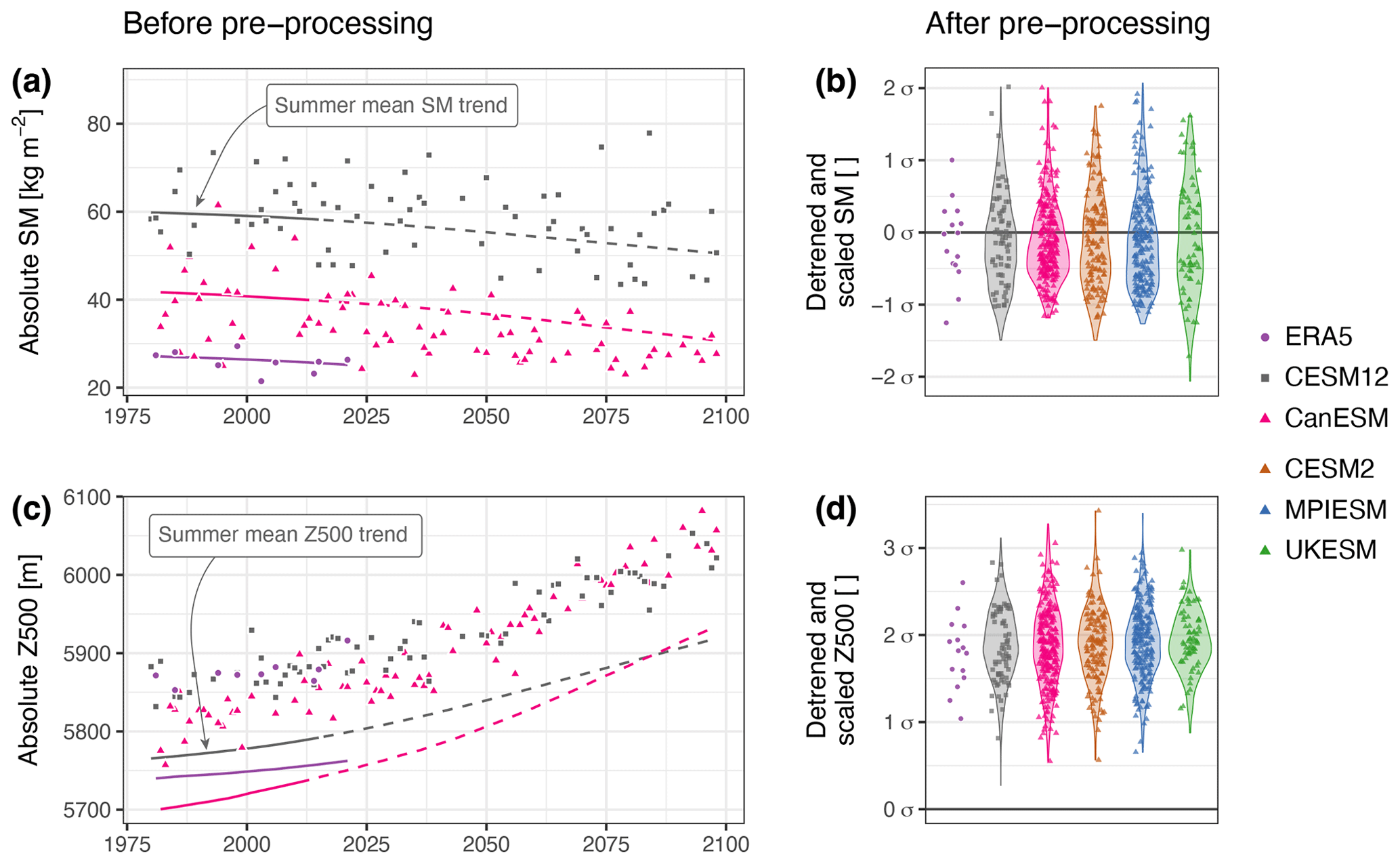
Figure 1Unprocessed SM (a) and Z500 (c) values (points) during Tx7d events in the PNW area for CESM12, CanESM (ensemble members 1 to 3, omitting other models and ensemble members for visibility) and ERA5. Estimated summer mean SM (a) and Z500 (c) GMST forced trends (solid lines: historical and reanalysis forcing, dashed lines: trend in a future RCP-8.5 or SSP5-8.5 climate scenario). Predictor data distributions of xSM (b) and (d) after pre-processing (detrending and scaling) across all datasets (violin plot) and individual event data (points) shown in panels (a) and (c). No violin distribution is shown for ERA5 due to the limited sample size.
Figure 1b and d demonstrate good agreement in the distribution of pre-processed SM and Z500 predictors across climate model and ERA5 reanalysis data, with a similar mean and variance. Figure 2a further confirms that the average geopotential height anomaly fields of the CESM12 and ERA5 datasets compare well, and there is also good agreement between the six leading principal component patterns (eigenvectors) at the PNW location (Fig. 2b). An extended evaluation of predictand and predictor variables with respect to seasonality and the stationarity in variable means and variance over time is provided in Supplement Sect. S1.3.
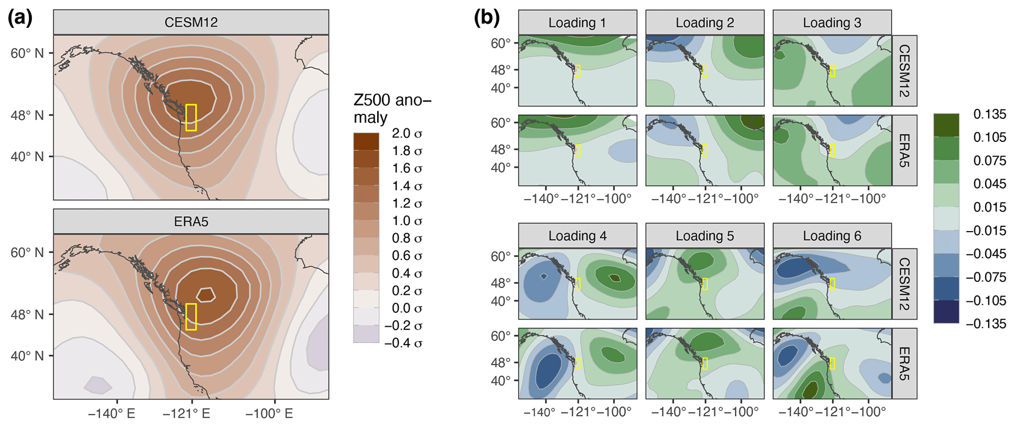
Figure 2(a) Average detrended and scaled Z500 anomaly fields in CESM12 (upper panel) and ERA5 (lower panel) during 5-year maximum temperature events relative to average summer Z500 conditions expressed in standard deviations. (b) The leading six principal component loading patterns of the detrended and scaled Z500 anomaly fields in CESM12 and ERA5. The area of interest is marked with a yellow box.
Statistical theory provides various concepts which are specifically tailored to the analysis of extreme values in a larger dataset, following the philosophy of “letting the tail speak for itself” (Cooley et al., 2019, p. 153). Two prominent methods in climate science are the block-maximum and peak-over-threshold approaches, both closely related within the framework of extreme value theory (Coles, 2001; de Haan and Ferreira, 2006). The former is often applied in the context of heatwave research, the primary reason being that temperature extremes are subject to seasonality, which is implicitly accounted for when analysing maxima of (multi-)annual blocks. The statistical distribution used to model block maxima is the generalised extreme value (GEV) distribution, a max-stable distribution with a similar theoretical justification to the Gaussian distribution for average values. Furthermore, the flexibility of the GEV allows for a natural treatment of non-stationarity in heat extremes, as GEV parameters can be formulated as functions of covariates, which are representative of heatwave drivers. Non-stationary GEV formulations based on global temperature or greenhouse gas forcing proxies were adopted for climate model evaluation (e.g. Wehner, 2020), analyses of return period changes in heat extremes (e.g. Zwiers et al., 2011; Huang et al., 2016), or extreme event attribution (e.g. Vautard et al., 2020; Philip et al., 2022). Considering its applicability to block maxima and the ability to account for non-stationarity in maxima driven by external covariates, the GEV provides the necessary capabilities to statistically quantify the effect of the selected physical process variables GMST (xGMST), SM (xSM) and the Z500 field () on the intensity of 5-year temperature maxima (yTx7d). Similar applications of non-stationary extreme value modelling with event-specific covariates are found in the literature, e.g. to investigate drivers of wind gust intensity (Friederichs et al., 2009) and surface level ozone (Eastoe and Tawn, 2009; Russell et al., 2016).
3.1 The non-stationary GEV model
The non-stationary GEV distribution in Eq. (1) is characterised by its three parameters: the non-stationary location parameter μ(t)∈ℝ (controlling the location of the distribution), the non-stationary scale parameter (controlling the width of the distribution) and the shape parameter ξ∈ℝ (controlling the tail characteristics of the distribution):
where . The location and scale parameters are functions of the covariates which represent the process variables prevalent in a specific event t. As a consequence, the distribution and corresponding metrics like quantiles or exceedance probabilities are always conditional on the state of the covariate set, which enters the location parameter μ(t) as follows:
We model the location parameter μ(t) in Eq. (2) as the sum of a constant intercept μ0 and a time-varying effect μ*(t), which is the sum of , and , all in unit degrees Celsius. The effect terms are linear functions of time-varying predictor variables GMST (xGMST), SM (xSM) and the Z500 field (), analogous to standard multivariate linear regression. For example, assuming a coefficient value μGMST=1.5 ∘C ∘C−1, a GMST anomaly of xGMST(t)=2 ∘C results in a GMST effect of ∘C, shifting the location parameter μ(t) and therefore the overall GEV distribution by +3 ∘C. In the following sections, changes in heatwave intensity refer to changes in the location parameter as a function of the predictors GMST, SM and the Z500 field, i.e. the combined effect μ*(t) of the physical process variables. The baseline value for the location parameter corresponds to average pre-industrial conditions, where the GMST, Z500 and SM effects are all zero (, i.e. μ(t)=μ0). It should be noted that this does not correspond to average summer conditions but to average conditions in 5-year summer temperature maxima associated with a distinct anti-cyclonic circulation pattern (shown in Fig. 2a). The coefficients estimated from data are therefore the intercept μ0 (∘C), μGMST (∘C ∘C−1), μSM and the coefficient vector μZ (∘C SD−1). The latter relates the standardised Z500 anomaly value at each grid point to the overall Z500 effect as a scalar product of the two vectors. Other methods quantify the Z500 or sea level pressure anomaly pattern effect on extreme temperature using weather classifications and circulation indices (Schaller et al., 2018), circulation analogues (Jézéquel et al., 2018; Terray, 2021), canonical correlation analysis (Della-Marta et al., 2007a), ridge regression (Sippel et al., 2019) or quantile regression forest (Vignotto et al., 2020).
The scale parameter σ(t) in Eq. (3) is modelled as a function of the non-stationary location parameter μ*(t), where a natural-logarithm link function ensures that the scale parameter stays strictly positive. This formulation allows the distribution to account for variability differences (heteroscedasticity) of temperature maxima yTx7d under varying conditions (Risser and Wehner, 2017; Robin and Ribes, 2020). As the variation in the location parameter is primarily governed by the changes in GMST, the scale parameter also primarily adjusts to different warming levels. Under average pre-industrial conditions (i.e. μ(t)=μ0), the scale parameter has the value σ(t)=exp(σ0).
The shape parameter ξ is constant and not a function of any process variables, which is general practice in similar studies (e.g. Philip et al., 2020). A non-stationary shape parameter would increase the variance in all estimates, considering that shape parameter estimates are associated with large uncertainties (Friederichs, 2010; Cooley, 2013).
3.2 Parameter estimation and regularisation
In order to adequately sample the upper tail of the temperature distribution, a 5-year block size was found to be required, considering the extensive autocorrelation in temperature data and the short summer period when temperatures peak (an extended discussion of the block size is provided in Supplement Sect. S2.1). Five-year block-maximum events were extracted from the period 1980–2089 as training data of the GEV models, events from stationary simulation periods (pre-industrial and historical 1850–1900) were used to obtain optimal starting values for the Z500 coefficients μZ (Supplement Sect. S2.2), and the last decade (2090–2100) was held out for validation purposes (see Sect. 3.3). This amounts to 3155 heatwave events available for parameter estimation in the largest dataset (CESM12; cf. Table 1) and 527 events in the smallest dataset (CESM2).
For the GEV model in Eq. (1) – with the full Z500 anomaly field as input – the number of parameters to be estimated is large (534 in total, thereof 528 in the coefficient vector μZ for the Z500 predictor field), and Z500 information across neighbouring grid points is significantly correlated, having adverse effects in the estimation procedure. The large number of highly correlated predictors can be accounted for by regularising the negative log-likelihood, specifically by adding a penalty term which increases with the sum of squared Z500 coefficients, i.e. the squared elements of vector μZ. This procedure is analogous to so-called ridge regression in statistical learning (e.g. Hastie et al., 2009) but explicitly accounts for the spatial structure of the Z500 grid. Confidence intervals (CIs) of parameter estimates are derived with parametric bootstrapping, drawing 600 percentile bootstrap samples of GEV parameters (Gilleland, 2020) also incorporating the uncertainty related to optimising the regularisation hyperparameter λ. More information on the implementation of the regularisation, selection of the optimal hyperparameter λ and retrieval of CIs is provided in Supplement Sect. S2.2. Given the advantages under non-stationary conditions (Katz, 2013), the regularised likelihood is optimised with numerical procedures implemented in the R software library extRemes (Gilleland and Katz, 2016).
3.3 Model evaluation
The GEV model with a location parameter as in Eq. (2) constitutes the full model, with all relevant process variables considered. The marginal improvement in predictive skill relative to models with fewer predictor variables is tested by also fitting the following two nested sub-models (with analogous parameterisation regarding the scale and shape parameter): the first still considers all three physical process variables but is only provided with the local Z500 information in the area of interest , analogous to the local SM information. The sub-model with parameterisation as in Eq. (4) is referred to as the local Z500 model:
Second, a further sub-model with only GMST as a covariate is estimated, which is referred to as the GMST-only model. The model formulation in Eq. (5) is representative of the standard non-stationary GEV model used in recent heatwave attribution studies (Kew et al., 2019; Vautard et al., 2020; Philip et al., 2022):
Model evaluation was conducted on a distinct testing period, 2090–2100, and a sub-set of events with a particularly strong Z500 effect (Fig 4a), in order to specifically test whether using the full Z500 field as a predictor (full model) adds value compared to local Z500 information only (local Z500 model). This second sub-set consists of all events with the 20 % highest estimated Z500 effect , sampled from both the training and testing periods (the “hat” notation refers to parameter estimates). The full model and the two sub-models (GMST-only and local Z500) are compared with two measures: first, the coefficient of determination R2, a standard model evaluation metric in statistical learning (Hastie et al., 2009; Wilks, 2011), which assesses the predictive quality in a regression context. The R2 score is not adjusted for the varying number of parameters in the models, as the parameters in the full model are heavily regularised. The predictive quality of the GMST-only model serves as the baseline for this score, and thus the respective R2 value is zero. Second, the continuous-ranked probability score (CRPS) (Wilks, 2011) is used to assess the overall fit of the GEV distribution with respect to the evaluation data. More information on how the scores are computed is provided in Supplement Sect. S2.3.
3.4 Post-estimation model adjustment
Applying a statistical model whose parameters were estimated from climate model data to specific heatwave events in reanalysis data implicitly assumes that the training (climate model) and evaluation (reanalysis) data share the same statistical characteristics. In this section, the necessary measures taken after model estimation are briefly summarised. The pre-processing (detrending and scaling) ensures that Z500 and SM predictors and xSM agree well across climate model and reanalysis data (see Fig. 1b and d). Differing GMST representations in climate models and reanalysis data were accounted for by expressing the GMST predictor as a relative anomaly to a fixed 1981–2010 average of 0.63 ∘C. Also, constant offsets in yTx7d values are corrected for, such that, of all GEV parameters, only the intercept parameter is adjusted. Supplement Sect. S2.4 outlines how the correction steps for differences in the GMST predictor and the Tx7d predictant are implemented. Reanalysis Z500 field data were also standardised, as the GEV parameters are also estimated based on standardised training data (see Sect. 2.2). Due to the limited availability of 5-year block maxima in reanalysis data, the multi-model Z500 field mean and standard deviation are used for the standardisation of reanalysis geopotential height fields.
In the following, the estimated parameters of the full GEV model are presented, which convey information on how the effects of physical process variables are found to alter the heatwave intensity. Furthermore, in the second part of this section, the relative improvement in the representation of temperature extremes by including the dynamical field (the full model) relative to using local process variables (local Z500 model) or GMST (GMST-only model) is assessed. The application of the statistical model to the PNW 2021 event is presented in the third part of the following section. For reference, a second application to a heatwave event at a different location (WRU) and simulated by a climate model is presented in Supplement Sect. S3.5.
Before drawing conclusions from a statistical model, it is vital to check whether the respective model is representative of the underlying data. Diagnostics like quantile–quantile plots in Supplement Sect. S3.1 confirm that the full GEV model is capable not only of describing the data used for estimating the respective parameters, but also performing reasonably on the testing dataset as well as for events with a dominant Z500 effect.
4.1 Scaling estimates of process variables
The linear and additive structure of the statistical model in Eq. (2) allows us to disentangle and quantify the relative contributions of physical process variables by the relative size of the associated location parameter terms. In the following, we discuss scaling relationships of extreme temperature with the respective predictor variables (e.g. the increase in Tx7d temperature in degrees Celsius as a result of a 1 standard deviation unit change in SM). These relationships are quantified by the coefficient estimates shown in Fig. 3 (estimates for locations WRU and WEU are shown in Supplement Figs. S18 and S19).
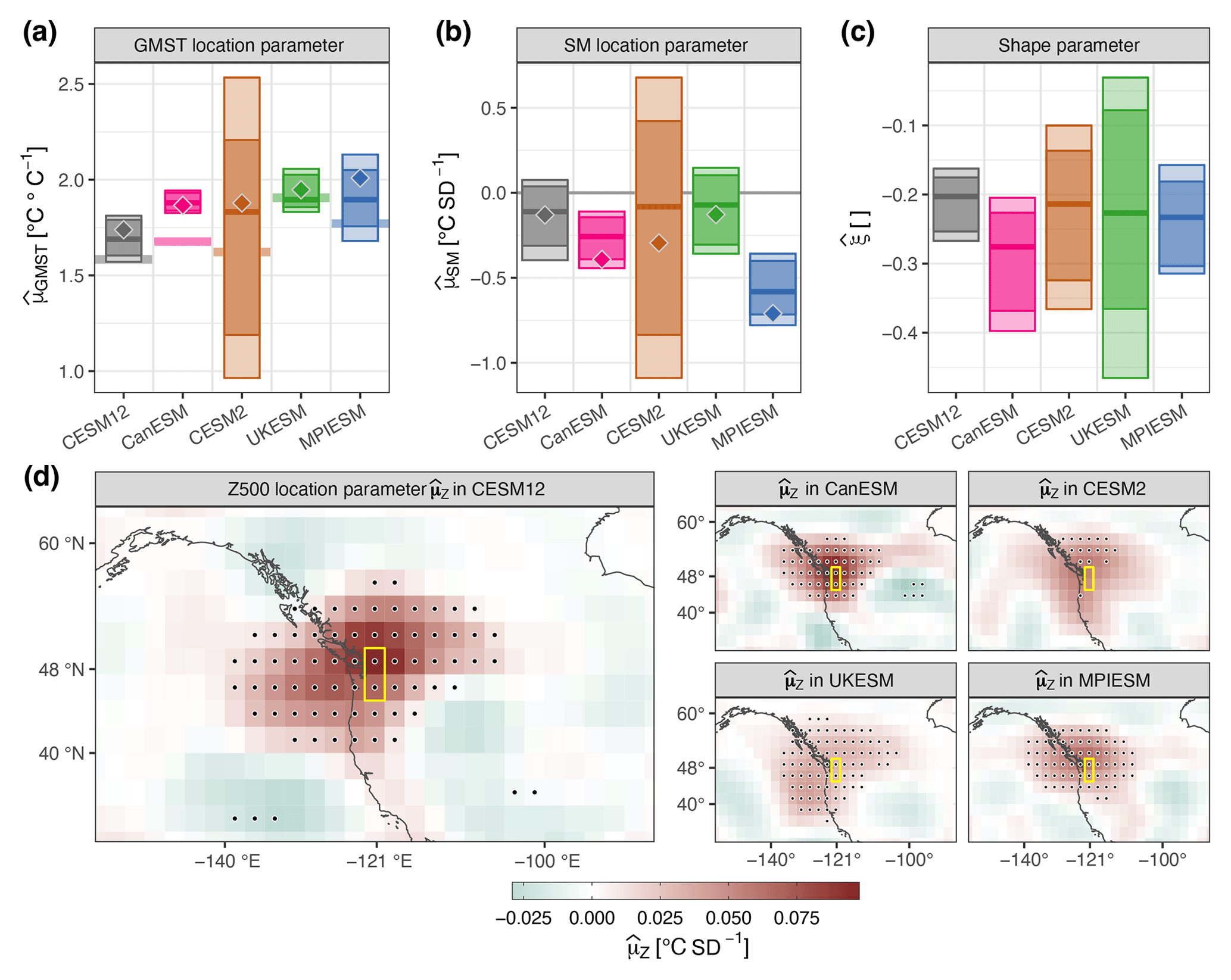
Figure 3GEV parameter estimates at the PNW location. Point estimates (central horizontal line in the box) and bootstrap 95 % (dark shading) and 99 % (light shading) CI of the (a) and (b) coefficients and (c) the shape parameter . The diamonds show linear regression estimates of the same coefficients, and the horizontal, semi-transparent bars show the linear regression scaling coefficient of summer mean temperature change with GMST. (d) Maps of estimated Z500 coefficients. Stippling marks coefficients for which the 99 % CI does not include zero.
4.1.1 Scaling with GMST
We first analyse the scaling relationship of local extreme and global average temperature, as this constitutes the dominating long-term thermodynamic effect on heatwave intensity. As linear detrending removed the global warming signal in the SM and Z500 covariates, the effect of global warming is solely represented by the GMST covariate xGMST. The estimates of the scaling coefficient in Fig. 3a indicate that heatwave extreme temperatures intensify at a rate of roughly 1.7 to 1.9 ∘C per 1 ∘C warming in GMST at the PNW location. A scaling value larger than unity should be expected, as land areas are subject to stronger warming relative to oceans (Sutton et al., 2007; Toda et al., 2021), and thus extreme temperature on land should increase at a higher rate than the global average used as a covariate. Similar scaling values are found when, instead of applying a non-stationary GEV model, a simple least-squares linear regression is used for the fit (diamonds in Fig. 3a). It should further be noted that, for all underlying climate model datasets, the scaling exceeds that of seasonal summer mean temperature scaling, shown as the horizontal bars in the background of Fig. 3a. This is an indication that the intensification of heatwaves outpaces the general seasonal warming rate, a phenomenon also found in observational data (Della-Marta et al., 2007b; Lorenz et al., 2019). Scaling factors reported by Seneviratne and Hauser (2020, Supplement Table S1, determined in CMIP5 and CMIP6 multi-model assessments at a 1.5 ∘C warming level) are slightly lower in western North America, with 1.47 in CMIP5 and 1.61 ∘C ∘C−1 in CMIP6. These lower scaling estimates might be due to differences in event definitions, as Seneviratne and Hauser (2020) analyse annual single-day temperature maxima which are spatially averaged over a substantially larger area. The relatively large CI of the CESM2 model can be explained by the fact that it consists of only five ensemble members and thus provides fewer data.
4.1.2 Scaling with SM
The estimates in Fig. 3b show a negative association of soil moisture anomalies with extreme temperature, implying that dry surface conditions are favourable for more intense heatwave events, in accordance with the literature (Fischer et al., 2007; Miralles et al., 2014). However, for three climate model datasets, the effect is statistically insignificant, as the CIs include zero. The pattern is again comparable to linear regression scaling estimates, even though these indicate a more negative scaling relationship. Weaker and non-significant scaling relationships at the PNW location estimated with the full GEV model may be due to several factors: first, the SM covariate is a weighted average of SM in the previous and current months of the heatwave event and is thus potentially also affected by precipitation events after the heatwave event. Suarez-Gutierrez et al. (2020) discuss the advantages and disadvantages of considering SM in the months previous to the extreme and during the extreme as predictors. Second, a linear detrending of SM with respect to global warming might not capture non-linear changes in soil moisture regimes (Seneviratne et al., 2010) and thus further disturb the signal of SM in heatwave intensity. Third, SM information is obtained for soil depths of roughly 20 cm, as soil layer definitions vary across land models. For the given depth, the signal might be larger or smaller, depending on the respective location. The negative scaling signal is stronger and more consistent in the WRU and WEU study areas (Supplement Figs. S18 and S19), in accordance with Zschenderlein et al. (2019), who find temperature extremes in these regions to be governed by near-surface advection and diabatic heating and thus potentially more affected by surface conditions compared to the PNW area.
4.1.3 Scaling with Z500
The spatially resolved effect of the geopotential height field on local extreme temperature is represented in the coefficient fields of in Fig. 3d. Estimates in the vicinity of the study area (yellow box) are generally positive and significantly different from zero, reflecting the fact that positive Z500 anomalies – corresponding to a high-pressure system – are a key driver of temperature extremes. Pfahl and Wernli (2012) show that between 40 % and 60 % of all 6-hourly warm temperature extremes in that region are associated with a co-located blocking event. However, the significance information is only approximate, as the bootstrapping procedure inherits the bias of the regularised estimates, and the significance information is not corrected for multiple testing. Thus the stippling should only be interpreted as a first-order approximation of statistical significance. Areas with (mostly non-significant) negative coefficients are located south-east and south-west of the grid points associated with (significant) positive coefficient estimates, resembling the omega blocking pattern (e.g. Detring et al., 2021), but the orientation and spatial extent vary across climate model datasets. It should also be noted that temporally integrated effects, for example the progressive accumulation of heat in a persistent atmospheric high-pressure situation (as described by Miralles et al., 2014), cannot be explicitly accounted for with this model, as only temporally co-occurring 7 d averaged geopotential height fields are analysed.
4.1.4 Scale and shape parameters
The log-scale parameter in Eq. (3) is a linear function of the location parameter, and thus it indirectly adjusts to heatwave processes, but primarily to GMST, as this predictor is responsible for the dominating long-term change in yTx7d. However, only for two climate model datasets, CESM12 and CanESM, is a significantly positive σ1 parameter estimated (not shown). This is in accordance with earlier studies finding only minor changes in GEV scale and shape parameters over historical and future periods (Wehner, 2020). Scale parameter intercepts are roughly 40 % larger in the nested GMST-only sub-model than the respective estimates of the full model, as substantially more variability is explained with the full Z500 predictor, which materialises in a narrower probability distribution (Jézéquel et al., 2018). The shape parameters ξ are estimated to be negative for all climate model datasets, ranging from −0.28 to −0.20 (Fig. 3c), thus constraining the upper bound of the probability distribution to an estimated non-stationary maximum value of . For the sub-models, shape parameters are generally estimated to be higher (−0.18 to −0.10), indicating that including the Z500 field information constrains the variability in the tail of the distribution.
In summary, the estimated parameters associated with the process variables are consistent with physical understanding and earlier research. However, it is not per se evident whether the model is missing additional crucial predictor information and whether the linear additive model structure can represent the relationship between predictors and predictant. In Supplement Sect. S3.2 the potential effects of seasonality and low-frequency climate variability on Tx7d data are analysed. No relevant signal could be detected, except for a tendency to overestimate the intensity of heat extremes at the end of the summer period, indicating that all relevant first-order process variables are considered.
With respect to the model structure, prior process understanding and sufficient data provide the basis and justification for a non-stationary modelling approach (Koutsoyiannis and Montanari, 2015), always considering the related challenges (Serinaldi and Kilsby, 2015). With respect to the GMST covariate, an approximately linear scaling relationship has been demonstrated for CMIP5 and CMIP6 models across various mid-latitude locations (Seneviratne and Hauser, 2020). Supplement Fig. S20a also confirms that a GEV model with non-linear capabilities (a generalised additive extreme value model; see Youngman, 2022) predicts an almost linear relationship between Tx7d and GMST. Modelling a joint Z500–SM effect with the generalised additive approach also does not reveal any non-linear interaction which would have to be considered in order to adequately model heatwave intensity (Supplement Fig. S20b). The linear additive model structure is therefore sufficient in representing the effects of the physical process variables on heatwave intensity.
4.2 Statistical model skill evaluation
An interpretation of the GEV parameter estimates of the full GEV model is provided in the previous section. It remains to be shown that this complex model adds value compared to simpler model structures, i.e. with fewer predictor variables. We evaluate the full GEV model with respect to the local Z500 and GMST-only nested sub-models, based on skill score metrics introduced in Sect. 3.3. These scores are calculated for the training period (1980–2089), an independent testing period (2090–2099) and specific events across both the training and testing periods, where a strong Z500 effect is estimated as visualised in Fig. 4a. A summary of the R2 skill score metric across statistical models fitted to all considered climate model datasets and three locations (PNW, WEU and WRU) is shown in the top row of Fig 4b, where the GMST-only model serves as a baseline (and thus the respective R2 scores are zero). The bottom row of Fig 4b shows the respective summary for the CRPS skill score. A detailed discussion of skill score selection and results and an assessment of individual locations and climate model datasets are provided in Supplement Sect. S3.3 and S3.4, respectively.
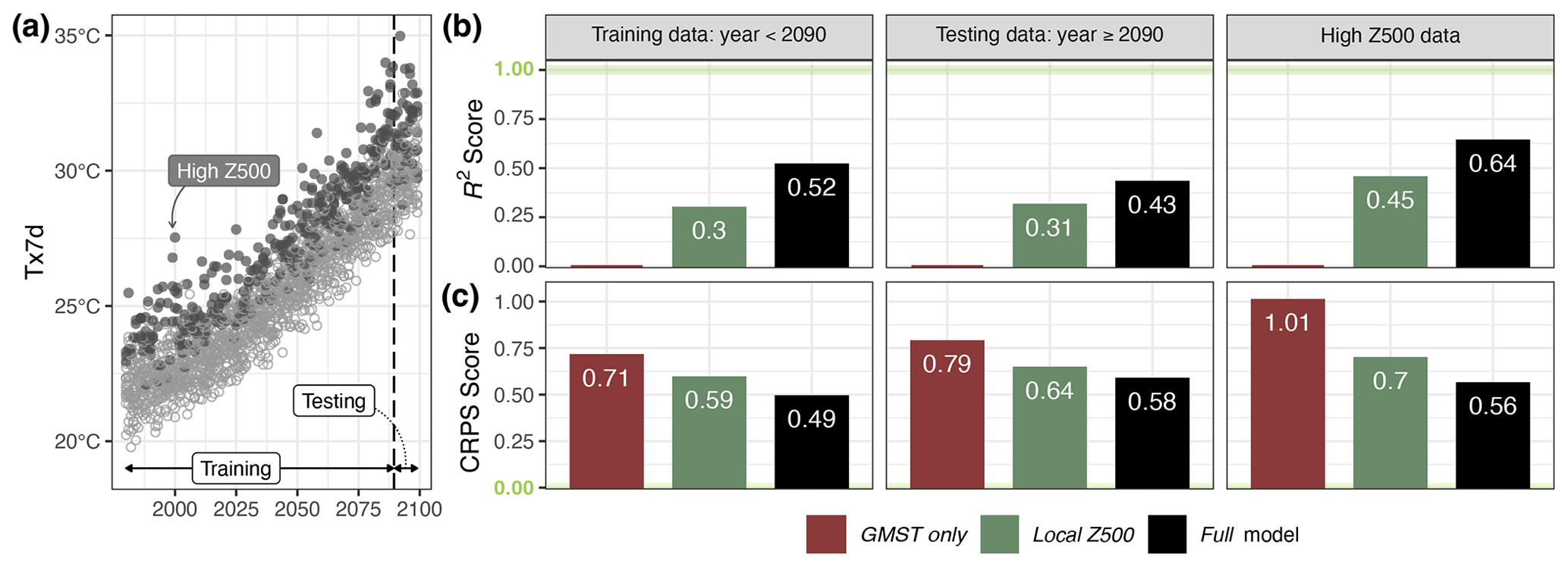
Figure 4(a) Scatter plot of predictant values yTx7d in CESM12, showing the training and testing periods and selected events with a strong Z500 effect. Average (b) R2 and (c) CRPS skill score values across climate model datasets for the training data (1980–2090), testing data (not used for model training, 2090–2100) and events with a strong Z500 effect (i.e. where the respective Z500 effect is among the 20 % strongest Z500 effects). For R2, the GMST-only model serves as the baseline, and thus the respective R2 score is zero. The horizontal light-green line marks the optimal “perfect” model score (R2=1 and CRPS=0).
Overall, the skill of the full model is higher from the regression perspective, indicated by higher average coefficient of determination R2 values than attained by the nested local Z500 and GMST-only sub-models, and it has better probabilistic coverage, indicated by lower average CRPS values than found for the nested sub-models. The ranking of scores remains consistent for individual models, but for the UKESM1-0-LL (UKESM) dataset, full model scores indicate slightly lower skill than the local Z500 model on testing data. Thus, it can be concluded that, in general, relevant information can be gained by considering the geopotential height field instead of just local Z500 anomalies in order to quantify the dynamic contribution to heatwave intensity.
4.3 Characterisation of the Pacific Northwest 2021 heatwave
The parameter estimates of the statistical GEV model discussed in Sect. 4.1 provide insight into the general relationship of the selected process-based covariates GMST, SM and Z500 with Tx7d. In the following, the GMST-only model and the full model are evaluated for the PNW heatwave of 2021, based on the respective ERA5 reanalysis data. For reference, we also provide an analogous analysis of a simulated heatwave event in the CESM12 large ensemble dataset in western Russia (i.e. not the actual 2010 heatwave event), which is presented in Supplement Sect. S3.5.
In the first step, we present the state of the physical process variables pre-conditioning the heatwave event, and given the estimated statistical models, the respective effect size is quantified. In the second step, the conditional event intensity is put into perspective: for instance, according to the statistical model, how would the intensity change at a different warming level? In the third step, an assessment of the respective likelihood changes is also presented. The following section will not just discuss the added value of the method, but also provide a critical review of its limitations.
4.3.1 Disentanglement of process contributions
The Pacific Northwest heatwave in late June 2021 was an unprecedented event considering the location and time of occurrence (Overland, 2021; Philip et al., 2022; Bercos‐Hickey et al., 2022; White et al., 2023), with 30.7 ∘C average temperature over 7 d exceeding all previous maxima in the ERA5-Land record (Fig. 5a). An unusually strong blocking anti-cyclone dominated the tropospheric circulation, driven by upstream wave activity (Neal et al., 2022; Schumacher et al., 2022). The centre of the Z500 anomaly is located north of the study region (Fig. 5c), with a magnitude substantially higher than observed for average Tx7d events (Fig. 2a). There is consensus that the larger western North American region was also affected by drought conditions (Bartusek et al., 2022; Schumacher et al., 2022); however, monthly weighted average SM values in the study domain were not anomalous relative to expected summer mean SM conditions (Fig. 5b). In addition to differences in the spatio-temporal definition, this might be explained by the seasonal decrease in SM over summer, implying that the specific anomaly value of 2021 was close to average due to the early occurrence of the event.
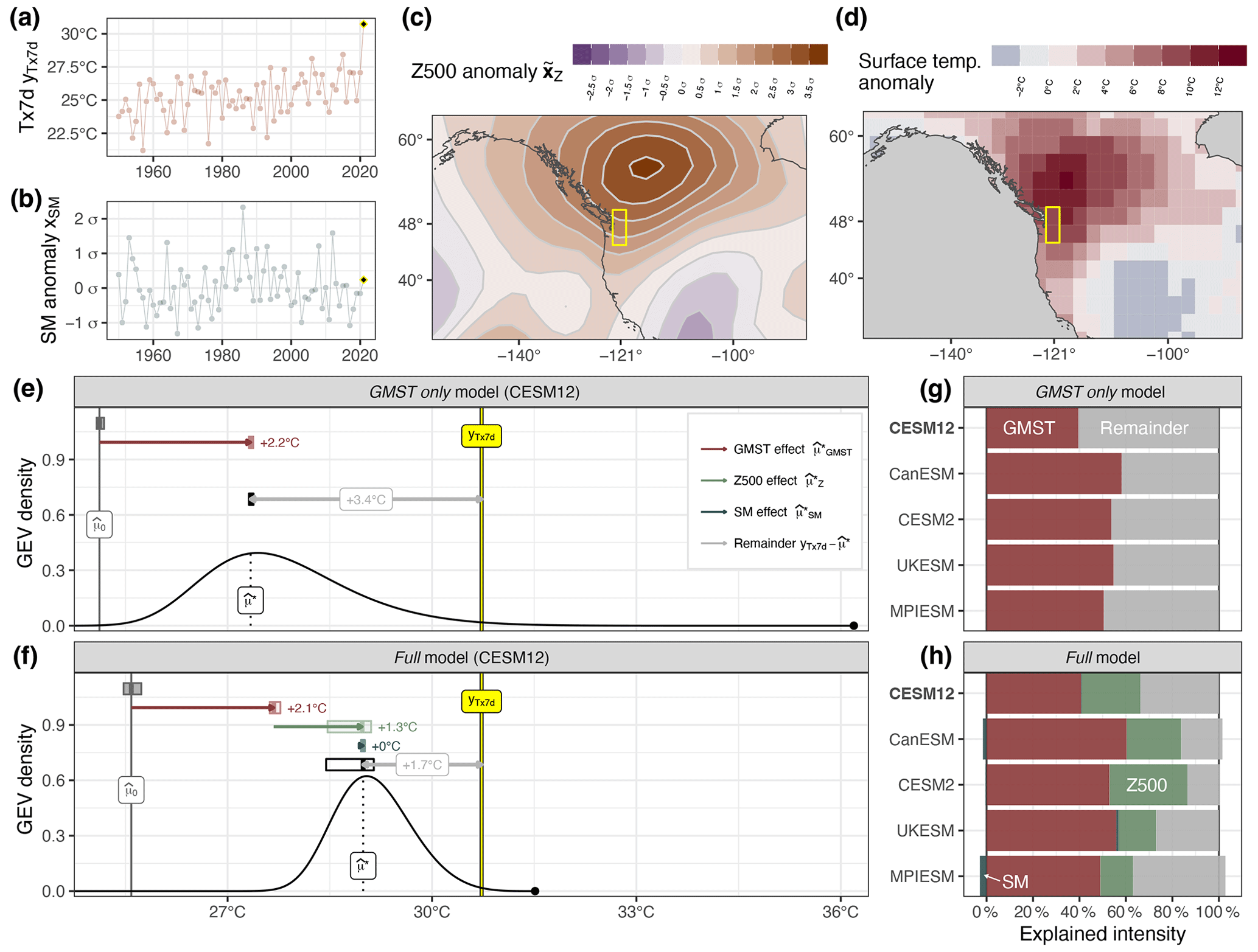
Figure 5ERA5-Land (a) 1-year Tx7d time series yTx7d and (b) corresponding detrended and scaled soil moisture anomalies xSM; the yellow point marks the PNW heatwave event. (c) Detrended and standardised ERA5 Z500 anomaly and (d) temperature anomaly fields of the respective event. Conditional GEV densities of the (e) GMST-only and (f) full models with estimated effect sizes (horizontal arrows) and 95 % CI (horizontal bars), event intensity yTx7d (vertical yellow line), intercept (vertical grey line) and location parameter (vertical dotted line). Multi-model assessment of the relative effect sizes of (g) the GMST-only model and (h) the full GEV model.
As the PNW 2021 event falls into a period of strong global warming, the GMST effect amounts to ∘C (Fig. 5f), which can be interpreted as the expected intensification of Tx7d relative to a pre-industrial base state given the 2021 warming level. The relative contribution of this thermodynamic global warming effect (i.e. the explained difference between , which can be interpreted as the pre-industrial average heatwave intensity, and the observed event intensity yTx7d) is consistently estimated to fall between 40 % and 60 % across GEV models and the underlying climate model datasets (Fig. 5g and h). The estimated soil moisture effect is also consistently estimated to be negligible (since the input predictor value is close to zero), whereas the circulation effect is estimated to account for a significant fraction of intensity not explained by the GMST predictor variable. According to the CESM12-based GEV model, the Z500 effect amounts to ∘C (Fig. 5f), which is among the 7 % strongest Z500 effects found for all considered heatwave events simulated by the five climate models. The distribution of Z500 effect sizes and where the PNW 2021 event lies therein is shown in Fig. 6a. Overall, the total estimated effect size explained by the three process variables, i.e. the combination of GMST, Z500 and (negligible) SM effects, amounts to ∘C. For GEV models trained with CMIP6 climate model data, the respective estimates range from +2.9 (MPIESM) to +3.7 ∘C (CanESM and CESM2). The physical process variables thereby explain 60 %–80 % of the excess PNW 2021 heatwave intensity relative to average pre-industrial Tx7d events (Fig. 5h).
There remains a considerable gap between the estimated location parameter ∘C, which is the sum of the pre-industrial base state ( ∘C) and strong GMST and Z500 effects ( ∘C), and the observed event intensity of yTx7d=30.7 ∘C. This difference of 1.7 ∘C is referred to as the unexplained remainder term in Fig. 5f. Non-linear interactions of the land–atmosphere system and upstream latent heating were found to account for much of the intensity of the event (Philip et al., 2022; Mo et al., 2022; Schumacher et al., 2022; Bartusek et al., 2022), processes that are not represented in this linear statistical framework.
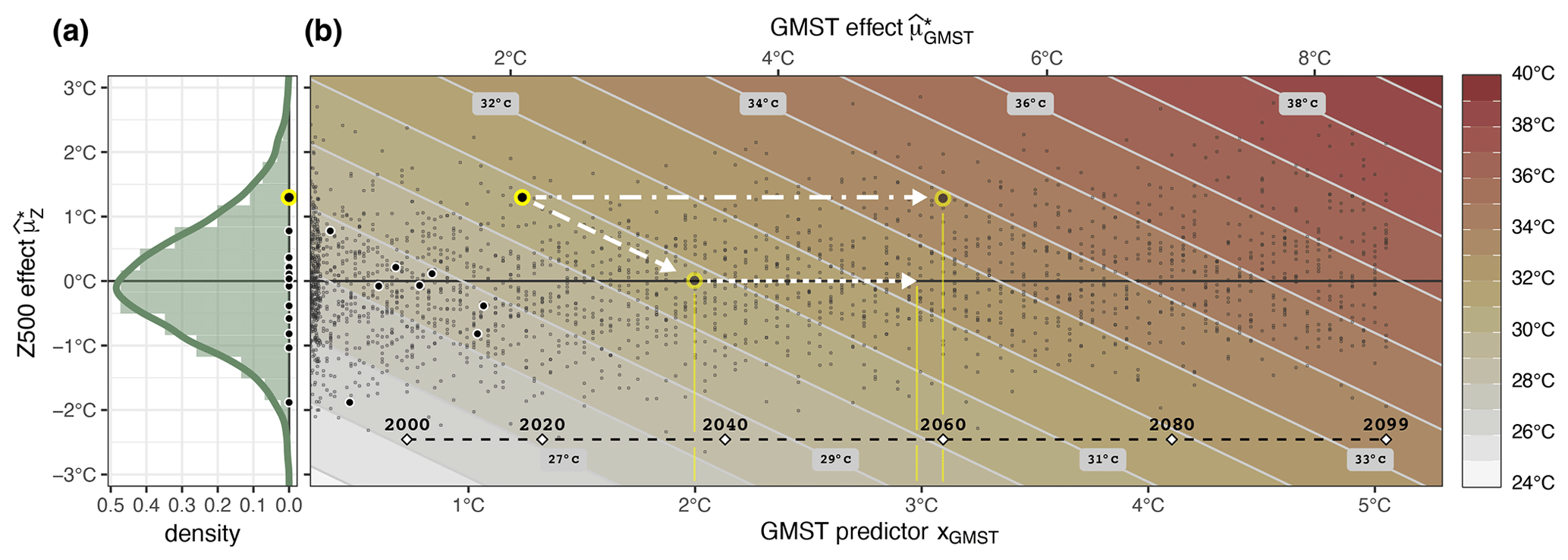
Figure 6(a) Density of Z500 effects on the abscissa in green (data of the CESM12 climate model dataset as a histogram and for all climate model datasets as smoothed density) at the PNW location. Dots indicate corresponding values in ERA5 5-year heatwave events, and the yellow dot shows the 2021 heatwave event. (b) Event intensity (coloured background) as a function of the GMST predictor xGMST (bottom ordinate) or the GMST effect (top ordinate) and the Z500 effect (on the abscissa, same as in panel (a)), conditional on the 2021 event-specific SM effect ∘C and unexplained remainder term of 1.73 ∘C (see Fig. 5f). The yellow dot marks the 2021 event under discussion, and further dots show 5-year heatwave events in the ERA5 reanalysis dataset (white dots) and the underlying CESM12 training and testing dataset (black dots). The locations of these points only refer to their respective GMST or Z500 effect, and their intensity is not related to the background colouring. The black dashed line at the bottom of the plot indicates the timing when certain GMST levels are reached in the CESM12 large ensemble under the RCP-8.5 forcing. White arrows and transparent yellow dots or lines refer to the “what if” scenarios discussed in the text.
Given the statistical model, how would the event intensity be altered under alternative prevalent conditions, in contrast to the actual drivers of the PNW heatwave? A major driver of the 2021 heatwave event is the anti-cyclone, whose effect is larger than in all previous 5-year ERA5 heatwave events (highest among the dots in Fig. 6a) but not far in the tail of all estimated Z500 effects found in the climate model datasets (histogram and density function in Fig. 6a). Eight events have Z500 effects of at least 3 ∘C, one even reaching 4.5 ∘C (Supplement Fig. S22), exceeding the estimated Z500 effect of the PNW 2021 event by 3.2 ∘C. If the event were to occur under the same conditions (in terms of Z500 and SM effects) and with the same unexplained event intensity in the year 2060 under the RCP-8.5 climate forcing, the temperature of an equivalent event would reach almost 34 ∘C (the dot–dashed white arrow in Fig. 6b).
The model also suggests that, in order to fully compensate for the Z500 effect, global temperatures would need to rise to roughly 2 ∘C (dashed arrow): that is, at a 2 ∘C warming level, the 2021 event would have the same conditional likelihood, even under average circulation conditions (of 5-year temperature maxima). Finally, if the global warming levels were to rise further by another 1 ∘C (dotted arrow), the unexplained remainder term would also be compensated for. Put differently, at this warming level, the event intensity of 2021 would be a standard 5-year heatwave extreme.
Our statistical model detects a considerable contribution of atmospheric circulation to the PNW 2021 heatwave intensity. Other methods used to disentangle the contribution of atmospheric circulation and warming to heatwaves include the analogue method (Yiou, 2014; Jézéquel et al., 2018) or targeted nudging experiments (Wehrli et al., 2019, 2022; Schumacher et al., 2022). The quantification of the circulation effect in the latter relies on the quantified temperature differences between the event and a reference climate and provides an upper bound of the circulation effect. The statistical method adopted here, on the other hand, provides a joint estimate of the event contribution but relies on a regression signal detectable in climate model heatwave events, thus probably rather providing a lower bound of the true circulation effect. The difficulty in detecting a signal is evident for SM in this example. The statistical models derive only a relatively weak relationship between SM anomalies and heatwave intensity (Fig. 3b), and furthermore, the SM anomaly retrieved for the PNW 2021 event is also small, and thus the method detects no SM effect. By adapting the SM definition to the respective circumstances (a different soil depth or spatial extent or using daily instead of monthly data), a stronger SM effect might be detected, but at the cost of an inevitable selection bias.
4.3.2 Conditional likelihood of the Pacific Northwest 2021 heatwave
The non-stationary GEV model also provides a (parametric) probability distribution quantifying the stochastic, unexplained variability in heat extremes, conditional on the respective process variables. In the following paragraphs, the conditional likelihood of the PNW heatwave is analysed, which is expressed in terms of its annual exceedance probability (AEP). The AEP is the probability of observing an event as intense or more intense than the PNW heatwave (according to the estimated GEV distribution and conditional on the respective covariates). Under stationary conditions, the AEP corresponds to the inverse of the return period. As the GEV distribution is derived from 5-year block maxima, the annual exceedance probability pex is obtained from the respective 5-year exceedance probability pex,5 as follows (see Supplement Sect. S2.5 for the derivation of the conversion formula):
If only GMST is considered as a driver for changing heatwave intensity – as in the GMST-only GEV model – the estimated AEP for a given Tx7d threshold can be displayed as a function over time. Figure 7 shows the respective exceedance probabilities based on the non-stationary GEV model estimated from CESM12 climate model data (white dots). The GEV probability density function shown in Fig. 5e corresponds to the cross section along the vertical dotted line. The non-linear increase in the location parameter (solid and dashed white lines) and the respective isolines of the AEP reflect the non-linear increase in GMST over time forced by an RCP-8.5 scenario. The GEV model captures the distribution of the CESM12 5-year block-maximum event intensity (small white dots) well, as these dots scatter around the line. Non-transparent large dots mark ERA5 heatwave events, which are shifted along the time coordinate to the year with equal GMST levels in the CESM12 climate model dataset (grey arrows).
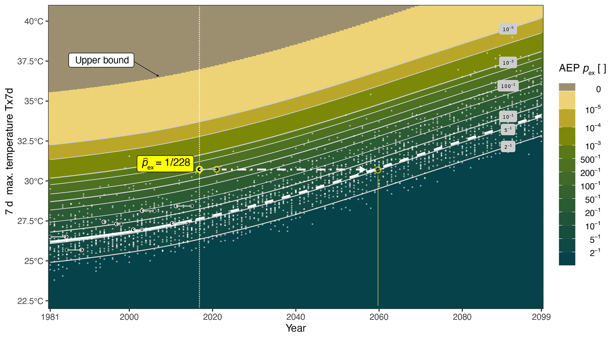
Figure 7AEP for heatwave intensity yTx7d (abscissa) as a function of the CESM12 model warming level in the respective model year (ordinate). Small white dots are events in the CESM12 climate model dataset, larger semi-transparent black dots with white strokes are ERA5 events in the year of occurrence, and non-transparent dots are the respective events shifted to the year of equal GMST as in the CESM12 climate model dataset (the 2021 PNW event has a yellow stroke). The vertical dotted line marks the cross section shown as a probability distribution in Fig. 5e. The bold white line marks the location parameter during the historical (solid) and RCP-8.5 (dashed) forcing periods, and the dot–dashed line is the “what if” scenario discussed in the text.
The estimated AEP value of the 2021 heatwave event is estimated to be ; thus, assuming constant 2021 global warming conditions, the 2021 event has an estimated return period of roughly 200 years. AEPs based on GEV distributions estimated from different climate model datasets range from to (Supplement Fig. S23). The spread partially reflects GEV model uncertainty but is likely dominated by uncertainty induced by the data-processing steps required to apply the statistical GEV framework estimated from climate model data to heatwave events in reanalysis data. The isoline reaches the Tx7d value of the PNW 2021 event roughly in 2060 (following the dot–dashed arrow in Fig. 7), and thus the corresponding event intensity becomes an average 5-year heatwave event at the respective warming level. This is well aligned with the finding in the previous Sect. 4.3.1 showing that compensating for the anomalous Z500 effect and the unexplained remainder term would require the warming level to increase to almost 3 ∘C, reached right before 2060 (following the dashed and dotted arrows in Fig. 6b).
Figure 6b visualises the change in intensity of the 2021 PNW for a specific combination of GMST and Z500 effects based on the full GEV model. For Fig. 8, the intensity yTx7d=30.7 ∘C is kept constant (as is the SM effect ∘C), and the resulting 2021 PNW event likelihoods for different hypothetical GMST and Z500 effect combinations are visualised. It is evident that, while the location parameter increases linearly in Fig. 6b, changes in AEP are highly non-linear. In analogy to the scenarios discussed in Fig. 6b, we find that, in order to compensate for the synoptic circulation effect, the warming level would have to increase to roughly 2 ∘C (moving along the diagonal dashed arrow), and it would become an average 5-year heatwave event once a warming level of almost 3 ∘C is reached (moving further along the dotted arrow). An event of the same intensity and with the same synoptic circulation conditions would have an AEP of less than 0.5 in 2060 (moving along the horizontal dot–dashed arrow) and thus would be exceeded every second year.
The conditional AEP estimated by the full model is lower than the AEP estimated by the GMST-only model with , which might seem contradictory. However, it should be noted that, with the additional predictors, the GEV model became more flexible and able to explain year-to-year variability, and thus the width of the distribution also decreased (see Fig. 5e and f). A smaller AEP thus means that the event intensity moved even further into the tail of the distribution, given the event-specific circumstances. Also, there is a large uncertainty associated with this estimate, which is underlined by the fact that conditional AEP estimates retrieved from full GEV models based on other climate model datasets range from to . Still, an interesting observation is that, according to the GEV models fitted to CESM12 and MPIESM data (not shown), the AEP of the 2021 event would be zero without the strong Z500 effect (i.e. under average Z500 conditions associated with 5-year heatwave intensity, following the vertical downward arrow in Fig. 8b). Thus, the strong anti-cyclone is recognised as a necessary condition for this specific heatwave event.
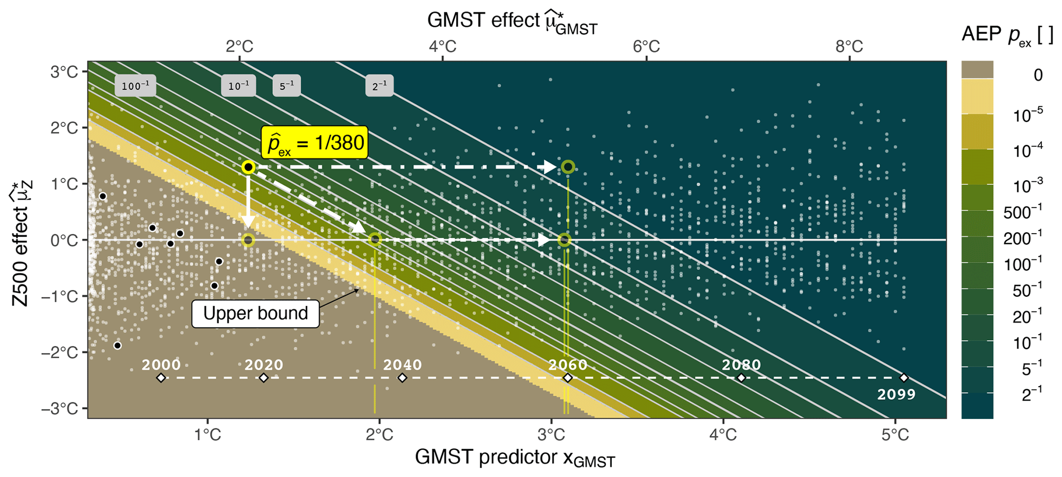
Figure 8AEP of the 2021 PNW event C (coloured background, with the soil moisture effect fixed at the 2021 value ∘C) as a function of GMST xGMST (bottom ordinate) or GMST forcing (top ordinate) and Z500 forcing (on the abscissa). Small white dots are 5-year heatwave events in the CESM12 climate model dataset, and larger dots are from the ERA5 reanalysis dataset. The line at the bottom of the plot indicates the timing when a certain GMST level is reached in the CESM12 large ensemble under the RCP-8.5 forcing. White arrows mark the “what if” scenarios discussed in the text.
The following limitations should be considered regarding conditional AEP estimates: first, non-stationary extreme value theory strictly holds only for slowly varying covariates (like the GMST covariate), such that block maxima arise from a larger set of observations which are identically distributed given the covariate (Cooley et al., 2019). This is not the case for the SM and Z500 covariates, as they vary at the same pace as the response variable yTx7d. Second, tail measures are highly sensitive and non-robust. Given for example the CI of effect sizes in Fig. 5f, it is evident that, shifting the distribution within the range of the CI (horizontal bar) of the location parameter , the exceedance probability (the area under the density curve beyond the yellow vertical line) changes substantially in response. Again, the merging of climate model and reanalysis data can also cause significant differences in the estimated AEP. Thus, the respective results must be interpreted as first-order estimates of the conditional event likelihood.
In this publication we introduce and evaluate a statistical framework to disentangle and quantify the effect of three major physical drivers of heatwave intensity and likelihood: the long-term warming trend, the regional-scale atmospheric circulation and local soil moisture anomalies. The respective relationships are integrated into a non-stationary extreme value model by estimating the respective parameters across a large set of heatwave events in long climate model simulations and large initial-condition ensembles. The framework is then applied to reanalysis data in order to estimate the respective contributions in observed heatwave events, specifically the 2021 Pacific Northwest heatwave. The climate change signal is first separated from the circulation and soil moisture covariates, such that a linear and additive model structure is representative of the statistical relationship of heatwave intensity with the considered process variables. It is shown that, by detrending and scaling, the covariates become comparable in mean and variance across climate model datasets. Thus, the pre-processing allows the relationship structure learned in climate model simulations to be transferred to heatwave events in reanalysis data. The statistical model benefits from the regional circulation field information by pre-training parameters in a stationary pre-industrial environment and regularising the respective estimates, thus guarding against overfitting.
Estimated GEV parameters provide valuable information on the relationship of local extreme temperatures with global warming, indicating that heatwave events intensify beyond the summer mean temperature trends. In the case of the PNW area, the 7 d annual temperature maxima increase by almost 2 ∘C per degree of global warming. The circulation contribution is largest for positive geopotential height anomalies in the vicinity of the study area, where clear-sky conditions and subsidence locally affect surface temperatures. Even though this indicates that Z500 conditions close to the heatwave centre are important, the statistical model accounting for the full circulation field outperforms the sub-model only based on very localised geopotential height information, explaining an additional 12 % of extreme temperature variability in an independent testing period.
For the PNW 2021 heatwave event, the dominant contribution of the anti-cyclone and the amplification by global warming is confirmed by our analysis. The event magnitude is estimated to be increased by 2.1 ∘C through global warming relative to pre-industrial conditions, and 43 % of the remaining event intensity is directly linked to the circulation pattern. However, a substantial fraction of the total event intensity is not explained by the statistical model, suggesting that non-local processes such as diabatic heating, which are not accounted for by this approach, have contributed substantially to the record-breaking temperatures. Given the conservative regularisation strategy, we interpret the estimated effect sizes associated with the respective covariates as a lower bound of the overall contribution of regional circulation and local land surface conditions.
The statistical model is also a tool to approach “what if” questions, such as by how much the event would intensify given the same dynamic conditions but at a different warming level or how much additional warming is needed for the same event intensity to occur under average circulation conditions. Changes in the exceedance probability under varying large- and regional-scale conditions can also be assessed. For instance, we estimate that the additional warming at a 2 ∘C GMST level would already compensate for the explained effect of the very anomalous PNW circulation conditions. Based on our framework, we can further demonstrate that, without the exceptional circulation conditions, the respective event intensity could not be reached. While these estimates are associated with substantial uncertainties, they provide interesting insights into the strongly non-linear dependence of event likelihood on global warming levels, where comparatively small increases in global mean temperature drastically increase the exceedance probability of former tail events.
Given the capabilities and limitations of the method, it can serve as an additional tool to characterise and assess both simulated and observed low-likelihood heatwave extremes. The method can further be extended by not just applying the model to observational data, but also integrating it into the estimation procedure, such that the distribution estimated from climate model data is also constrained by observations (Gabda et al., 2019; Robin and Ribes, 2020). Our approach can provide an additional line of evidence for attributing an extreme event not only to anthropogenic climate change, but also to regional circulation and local land surface conditions, thus helping to put future extreme events into a refined risk-based context (Stott et al., 2016). Even though the statistical model is fundamentally probabilistic in nature, its capability to answer “what if” questions may also serve as a basis for process-based storyline analyses (Shepherd, 2016).
All original CMIP6, ERA5 and ERA5-Land reanalysis data used in this study are publicly available.
-
CMIP6: https://esgf-node.llnl.gov/projects/cmip6/ (WCRP, 2023; Eyring et al., 2016)
-
ERA5: https://doi.org/10.24381/cds.adbb2d47 (Hersbach et al., 2023)
-
ERA5-Land: https://doi.org/10.24381/cds.e2161bac (Muñoz Sabater, 2019)
Pre-processed data (including CESM12 large ensemble model data) are available at https://doi.org/10.3929/ethz-b-000615056 (Zeder and Fischer, 2023). Code for pre-processing of data, reading the pre-processed data and GEV model training and event analysis is available at https://git.iac.ethz.ch/climphys/climate-extremes/nonstationary-extremes (last access: 11 July 2023). Regularised GEV code is available at https://git.iac.ethz.ch/climphys/climate-extremes/regextremes (last access: 11 July 2023).
The supplement related to this article is available online at: https://doi.org/10.5194/ascmo-9-83-2023-supplement.
JZ: conceptualisation, data curation, methodology, software, formal analysis, writing, visualisation. EMF: conceptualisation, methodology, formal analysis, writing, supervision.
The contact author has declared that neither of the authors has any competing interests.
Publisher’s note: Copernicus Publications remains neutral with regard to jurisdictional claims in published maps and institutional affiliations.
We would like to thank the associate editor Likun Zhang, Jonathan Koh and three anonymous reviewers for their helpful and constructive feedback and suggestions. We further thank Christoph Frei for the discussion of GEV properties and scoring measures and Urs Beyerle, Ruth Lorenz and Lukas Brunner for the maintenance of the CESM and CMIP6 climate model data archive. We thank the World Climate Research Programme’s Working Group on Coupled Modelling, which is responsible for CMIP, and we thank the climate modelling groups for producing and making available the model output. We also thank all the scientists, software engineers and administrators who contributed to the development of CESM. The analysis was carried out in R (R Core Team, 2022), and thus we thank all the contributors to the numerous R packages which were crucial for this work.
This research has been supported by the Schweizerischer Nationalfonds zur Förderung der Wissenschaftlichen Forschung (grant no. 200020_178778) and the European Commission, Horizon 2020 (grant no. 101003469).
This paper was edited by Likun Zhang and reviewed by Jonathan Koh and three anonymous referees.
Akhtar, R.: Introduction: Extreme Weather Events and Human Health: A Global Perspective, in: Extreme Weather Events and Human Health, edited by Akhtar, R., Springer International Publishing, Cham, 3–11, https://doi.org/10.1007/978-3-030-23773-8_1, 2020. a
Barriopedro, D., Fischer, E. M., Luterbacher, J., Trigo, R. M., and García-Herrera, R.: The Hot Summer of 2010: Redrawing the Temperature Record Map of Europe, Science, 332, 220–224, https://doi.org/10.1126/science.1201224, 2011. a
Bartusek, S., Kornhuber, K., and Ting, M.: 2021 North American heatwave amplified by climate change-driven nonlinear interactions, Nat. Clim. Change, 12, 1143–1150, https://doi.org/10.1038/s41558-022-01520-4, 2022. a, b
Beillouin, D., Schauberger, B., Bastos, A., Ciais, P., and Makowski, D.: Impact of extreme weather conditions on European crop production in 2018, Philos. T. R. Soc., 375, 20190510, https://doi.org/10.1098/rstb.2019.0510, 2020. a
Bercos‐Hickey, E., O’Brien, T. A., Wehner, M. F., Zhang, L., Patricola, C. M., Huang, H., and Risser, M. D.: Anthropogenic Contributions to the 2021 Pacific Northwest Heatwave, Geophys. Res. Lett., 49, e2022GL099396, https://doi.org/10.1029/2022GL099396, 2022. a
Bieli, M., Pfahl, S., and Wernli, H.: A lagrangian investigation of hot and cold temperature extremes in europe, Q. J. Roy. Meteor. Soc., 141, 98–108, https://doi.org/10.1002/qj.2339, 2015. a
Brunner, L., Hauser, M., Lorenz, R., and Beyerle, U.: The ETH Zurich CMIP6 next generation archive: technical documentation, Tech. Rep., ETH Zurich, Institute for Atmospheric and Climate Science, Zurich, Switzerland, Zenodo, https://doi.org/10.5281/zenodo.3734128, 2020. a
Cleveland, R. B., Cleveland, W. S., McRae, J. E., and Terpenning, I.: STL: A Seasonal-Trend Decomposition Procedure Based on Loess, J. Off. Stat., 6, 3–73, 1990. a
Coles, S.: An introduction to statistical modeling of extreme values, Springer series in statistics, 3rd print edn., Springer, London, ISBN 978-1-85233-459-8, https://doi.org/10.1007/978-1-4471-3675-0, 2001. a
Cooley, D.: Return Periods and Return Levels Under Climate Change, in: Extremes in a Changing Climate: Detection, Analysis and Uncertainty, edited by: AghaKouchak, A., Easterling, D., Hsu, K., Schubert, S., and Sorooshian, S., chap. 4, Springer Netherlands, Dordrecht, Netherlands, 97–114, https://doi.org/10.1007/978-94-007-4479-0, 2013. a
Cooley, D., Hunter, B. D., and Smith, R. L.: Univariate and Multivariate Extremes for the Environmental Sciences, in: Handbook of Environmental and Ecological Statistics, edited by: Gelfand, A., Fuentes, M., Hoeting, J. A., and Smith, R. L., chap. 8, Chapman and Hall/CRC, Taylor & Francis, Boca Raton, 153–180, ISBN 9781315152509, https://doi.org/10.1201/9781315152509-9, 2019. a, b
Deb, P., Moradkhani, H., Abbaszadeh, P., Kiem, A. S., Engström, J., Keellings, D., and Sharma, A.: Causes of the Widespread 2019–2020 Australian Bushfire Season, Earth's Future, 8, e2020EF001671, https://doi.org/10.1029/2020EF001671, 2020. a
de Haan, L. and Ferreira, A.: Extreme Value Theory: An Introduction, Springer Science & Business Media, New York, NY, United States, ISBN 978-0-387-29959-4, https://doi.org/10.1007/0-387-34471-3, 2006. a
Della-Marta, P. M., Haylock, M. R., Luterbacher, J., and Wanner, H.: Doubled length of western European summer heat waves since 1880, J. Geophys. Res., 112, D15103, https://doi.org/10.1029/2007JD008510, 2007a. a
Della-Marta, P. M., Luterbacher, J., von Weissenfluh, H., Xoplaki, E., Brunet, M., and Wanner, H.: Summer heat waves over western Europe 1880–2003, their relationship to large-scale forcings and predictability, Clim. Dynam., 29, 251–275, https://doi.org/10.1007/s00382-007-0233-1, 2007b. a, b, c
Deser, C., Terray, L., and Phillips, A. S.: Forced and internal components of winter air temperature trends over North America during the past 50 years: Mechanisms and implications, J. Climate, 29, 2237–2258, https://doi.org/10.1175/JCLI-D-15-0304.1, 2016. a
Detring, C., Müller, A., Schielicke, L., Névir, P., and Rust, H. W.: Occurrence and transition probabilities of omega and high-over-low blocking in the Euro-Atlantic region, Weather Clim. Dynam., 2, 927–952, https://doi.org/10.5194/wcd-2-927-2021, 2021. a
Domeisen, D. I. V., Eltahir, E. A. B., Fischer, E. M., Knutti, R., Perkins-Kirkpatrick, S. E., Schär, C., Seneviratne, S. I., Weisheimer, A., and Wernli, H.: Prediction and projection of heatwaves, Nature Reviews Earth & Environment, 4, 36–50, https://doi.org/10.1038/s43017-022-00371-z, 2022. a
Eastoe, E. F. and Tawn, J. A.: Modelling Non-Stationary Extremes with Application to Surface Level Ozone, J. R. Stat. Soc. C-Appl., 58, 25–45, https://doi.org/10.1111/j.1467-9876.2008.00638.x, 2009. a
Eyring, V., Bony, S., Meehl, G. A., Senior, C. A., Stevens, B., Stouffer, R. J., and Taylor, K. E.: Overview of the Coupled Model Intercomparison Project Phase 6 (CMIP6) experimental design and organization, Geosci. Model Dev., 9, 1937–1958, https://doi.org/10.5194/gmd-9-1937-2016, 2016. a, b
Feudale, L. and Shukla, J.: Influence of sea surface temperature on the European heat wave of 2003 summer. Part I: an observational study, Climate Dynamics, 36, 1691–1703, https://doi.org/10.1007/s00382-010-0788-0, 2011. a
Fischer, E. M. and Schär, C.: Future changes in daily summer temperature variability: driving processes and role for temperature extremes, Clim. Dynam., 33, 917–935, https://doi.org/10.1007/s00382-008-0473-8, 2009. a
Fischer, E. M., Seneviratne, S. I., Vidale, P. L., Lüthi, D., and Schär, C.: Soil moisture-atmosphere interactions during the 2003 European summer heat wave, J. Climate, 20, 5081–5099, https://doi.org/10.1175/JCLI4288.1, 2007. a, b
Fischer, E. M., Sippel, S., and Knutti, R.: Increasing probability of record-shattering climate extremes, Nat. Clim. Change, 11, 689–695, https://doi.org/10.1038/s41558-021-01092-9, 2021. a, b
Fischer, P. H., Brunekreef, B., and Lebret, E.: Air pollution related deaths during the 2003 heat wave in the Netherlands, Atmos. Environ., 38, 1083–1085, https://doi.org/10.1016/j.atmosenv.2003.11.010, 2004. a
Friederichs, P.: Statistical downscaling of extreme precipitation events using extreme value theory, Extremes, 13, 109–132, https://doi.org/10.1007/s10687-010-0107-5, 2010. a
Friederichs, P., Göber, M., Bentzien, S., Lenz, A., and Krampitz, R.: A probabilistic analysis of wind gusts using extreme value statistics, Meteorol. Z., 18, 615–629, https://doi.org/10.1127/0941-2948/2009/0413, 2009. a
Gabda, D., Tawn, J., and Brown, S.: A step towards efficient inference for trends in UK extreme temperatures through distributional linkage between observations and climate model data, Nat. Hazards, 98, 1135–1154, https://doi.org/10.1007/s11069-018-3504-8, 2019. a
Gessner, C., Fischer, E. M., Beyerle, U., and Knutti, R.: Very rare heat extremes: quantifying and understanding using ensemble re-initialization, J. Climate, 34, 6619–6634, https://doi.org/10.1175/JCLI-D-20-0916.1, 2021. a
Ghil, M., Yiou, P., Hallegatte, S., Malamud, B. D., Naveau, P., Soloviev, A., Friederichs, P., Keilis-Borok, V., Kondrashov, D., Kossobokov, V., Mestre, O., Nicolis, C., Rust, H. W., Shebalin, P., Vrac, M., Witt, A., and Zaliapin, I.: Extreme events: dynamics, statistics and prediction, Nonlin. Processes Geophys., 18, 295–350, https://doi.org/10.5194/npg-18-295-2011, 2011. a
Gilleland, E.: Bootstrap Methods for Statistical Inference. Part I: Comparative Forecast Verification for Continuous Variables, J. Atmos. Ocean. Tech., 37, 2117–2134, https://doi.org/10.1175/JTECH-D-20-0069.1, 2020. a
Gilleland, E. and Katz, R. W.: ExtRemes 2.0: An extreme value analysis package in R, J. Stat. Softw., 72, 1–39, https://doi.org/10.18637/jss.v072.i08, 2016. a
Hastie, T., Tibshirani, R., and Friedman, J.: The Elements of Statistical Learning, Springer Series in Statistics, Springer New York, New York, NY, https://doi.org/10.1007/b94608, 2009. a, b
Hersbach, H., Bell, B., Berrisford, P., Hirahara, S., Horányi, A., Muñoz-Sabater, J., Nicolas, J., Peubey, C., Radu, R., Schepers, D., Simmons, A., Soci, C., Abdalla, S., Abellan, X., Balsamo, G., Bechtold, P., Biavati, G., Bidlot, J., Bonavita, M., De Chiara, G., Dahlgren, P., Dee, D., Diamantakis, M., Dragani, R., Flemming, J., Forbes, R., Fuentes, M., Geer, A., Haimberger, L., Healy, S., Hogan, R. J., Hólm, E., Janisková, M., Keeley, S., Laloyaux, P., Lopez, P., Lupu, C., Radnoti, G., de Rosnay, P., Rozum, I., Vamborg, F., Villaume, S., and Thépaut, J. N.: The ERA5 global reanalysis, Q. J. Roy. Meteor. Soc., 146, 1999–2049, https://doi.org/10.1002/qj.3803, 2020. a
Hersbach, H., Bell, B., Berrisford, P., Biavati, G., Horányi, A., Muñoz Sabater, J., Nicolas, J., Peubey, C., Radu, R., Rozum, I., Schepers, D., Simmons, A., Soci, C., Dee, D., and Thépaut, J.-N.: ERA5 hourly data on single levels from 1940 to present, Copernicus Climate Change Service (C3S) Climate Data Store (CDS) [data set], https://doi.org/10.24381/cds.adbb2d47, 2023. a
Horton, D. E., Johnson, N. C., Singh, D., Swain, D. L., Rajaratnam, B., and Diffenbaugh, N. S.: Contribution of changes in atmospheric circulation patterns to extreme temperature trends, Nature, 522, 465–469, https://doi.org/10.1038/nature14550, 2015. a
Horton, R. M., Mankin, J. S., Lesk, C., Coffel, E., and Raymond, C.: A Review of Recent Advances in Research on Extreme Heat Events, Current Climate Change Reports, 2, 242–259, https://doi.org/10.1007/s40641-016-0042-x, 2016. a
Huang, W. K., Stein, M. L., McInerney, D. J., Sun, S., and Moyer, E. J.: Estimating changes in temperature extremes from millennial-scale climate simulations using generalized extreme value (GEV) distributions, Adv. Stat. Clim. Meteorol. Oceanogr., 2, 79–103, https://doi.org/10.5194/ascmo-2-79-2016, 2016. a
Hurrell, J. W., Holland, M. M., Gent, P. R., Ghan, S., Kay, J. E., Kushner, P. J., Lamarque, J. F., Large, W. G., Lawrence, D., Lindsay, K., Lipscomb, W. H., Long, M. C., Mahowald, N., Marsh, D. R., Neale, R. B., Rasch, P., Vavrus, S., Vertenstein, M., Bader, D., Collins, W. D., Hack, J. J., Kiehl, J., and Marshall, S.: The community earth system model: A framework for collaborative research, B. Am. Meteorol. Soc., 94, 1339–1360, https://doi.org/10.1175/BAMS-D-12-00121.1, 2013. a
IPCC: Summary for Policymakers, in: Climate Change 2021: The Physical Science Basis. Contribution of Working Group I to the Sixth Assessment Report of the Intergovernmental Panel on Climate Change, edited by: Masson-Delmotte, V., Zhai, P., Pirani, A., Connors, S., Péan, C., Berger, S., Caud, N., Chen, Y., Goldfarb, L., Gomis, M., Huang, M., Leitzell, K., Lonnoy, E., Matthews, J., Maycock, T., Waterfield, T., Yelekçi, O., Yu, R., and Zhou, B., Cambridge University Press, Cambridge, United Kingdom and New York, NY, USA, 3–32, https://doi.org/10.1017/9781009157896.001, 2021. a
Jahn, M.: Economics of extreme weather events: Terminology and regional impact models, Weather and Climate Extremes, 10, 29–39, https://doi.org/10.1016/j.wace.2015.08.005, 2015. a
Jézéquel, A., Yiou, P., and Radanovics, S.: Role of circulation in European heatwaves using flow analogues, Clim. Dynam., 50, 1145–1159, https://doi.org/10.1007/s00382-017-3667-0, 2018. a, b, c, d
Katz, R. W.: Statistical Methods for Nonstationary Extremes, in: Extremes in a Changing Climate: Detection, Analysis and Uncertainty, edited by: AghaKouchak, A., Easterling, D., Hsu, K., Schubert, S., and Sorooshian, S., chap. 2, Springer Netherlands, Dordrecht, Netherlands, 15–37, https://doi.org/10.1007/978-94-007-4479-0, 2013. a
Kew, S. f., Philip, S. Y., Jan van Oldenborgh, G., van der Schrier, G., Otto, F. E. L., and Vautard, R.: The Exceptional Summer Heat Wave in Southern Europe 2017, B. Am. Meteorol. Soc., 100, S49–S53, https://doi.org/10.1175/BAMS-D-18-0109.1, 2019. a
Koster, R. D., Guo, Z., Yang, R., Dirmeyer, P. A., Mitchell, K., and Puma, M. J.: On the Nature of Soil Moisture in Land Surface Models, J. Climate, 22, 4322–4335, https://doi.org/10.1175/2009JCLI2832.1, 2009. a
Koutsoyiannis, D. and Montanari, A.: Negligent killing of scientific concepts: the stationarity case, Hydrolog. Sci. J., 60, 1174–1183, https://doi.org/10.1080/02626667.2014.959959, 2015. a
Kröner, N., Kotlarski, S., Fischer, E., Lüthi, D., Zubler, E., and Schär, C.: Separating climate change signals into thermodynamic, lapse-rate and circulation effects: theory and application to the European summer climate, Clim. Dynam., 48, 3425–3440, https://doi.org/10.1007/s00382-016-3276-3, 2017. a
Lawrence, D. M., Oleson, K. W., Flanner, M. G., Thornton, P. E., Swenson, S. C., Lawrence, P. J., Zeng, X., Yang, Z.-L., Levis, S., Sakaguchi, K., Bonan, G. B., and Slater, A. G.: Parameterization improvements and functional and structural advances in Version 4 of the Community Land Model, J. Adv. Model. Earth Sy., 3, M03001, https://doi.org/10.1029/2011MS00045, 2011. a
Lehner, F., Deser, C., Maher, N., Marotzke, J., Fischer, E. M., Brunner, L., Knutti, R., and Hawkins, E.: Partitioning climate projection uncertainty with multiple large ensembles and CMIP5/6, Earth Syst. Dynam., 11, 491–508, https://doi.org/10.5194/esd-11-491-2020, 2020. a
Lorenz, R., Stalhandske, Z., and Fischer, E. M.: Detection of a Climate Change Signal in Extreme Heat, Heat Stress, and Cold in Europe From Observations, Geophys. Res. Lett., 46, 8363–8374, https://doi.org/10.1029/2019GL082062, 2019. a
Miralles, D. G., Teuling, A. J., van Heerwaarden, C. C., and Vilà-Guerau de Arellano, J.: Mega-heatwave temperatures due to combined soil desiccation and atmospheric heat accumulation, Nat. Geosci., 7, 345–349, https://doi.org/10.1038/ngeo2141, 2014. a, b
Mo, R., Lin, H., and Vitart, F.: An anomalous warm-season trans-Pacific atmospheric river linked to the 2021 western North America heatwave, Communications Earth & Environment, 3, 127, https://doi.org/10.1038/s43247-022-00459-w, 2022. a
Muñoz Sabater, J.: ERA5-Land hourly data from 1950 to present, Copernicus Climate Change Service (C3S) Climate Data Store (CDS) [data set], https://doi.org/10.24381/cds.e2161bac, 2019. a
Muñoz-Sabater, J., Dutra, E., Agustí-Panareda, A., Albergel, C., Arduini, G., Balsamo, G., Boussetta, S., Choulga, M., Harrigan, S., Hersbach, H., Martens, B., Miralles, D. G., Piles, M., Rodríguez-Fernández, N. J., Zsoter, E., Buontempo, C., and Thépaut, J.-N.: ERA5-Land: a state-of-the-art global reanalysis dataset for land applications, Earth Syst. Sci. Data, 13, 4349–4383, https://doi.org/10.5194/essd-13-4349-2021, 2021. a
Naveau, P., Hannart, A., and Ribes, A.: Statistical methods for extreme event attribution in climate science, Annu. Rev. Stat. Appl., 7, 89–110, https://doi.org/10.1146/annurev-statistics-031219-041314, 2020. a
Neal, E., Huang, C. S. Y., and Nakamura, N.: The 2021 Pacific Northwest Heat Wave and Associated Blocking: Meteorology and the Role of an Upstream Cyclone as a Diabatic Source of Wave Activity, Geophys. Res. Lett., 49, e2021GL097699, https://doi.org/10.1029/2021GL097699, 2022. a
Neale, R. B., Chen, C.-C., Gettelman, A., Lauritzen, P. H., Park, S., Williamson, D. L., Conley, A. J., Garcia, R., Kinnison, D., Lamarque, J.-F., Marsh, D., Mills, M., Smith, A. K., Tilmes, S., Vitt, F., Morrison, H., Cameron-Smith, P., Collins, W. D., Iacono, M. J., Easter, R. C., Ghan, S. J., Liu, X., Rasch, P. J., and Taylor, M. A.: Description of the NCAR Community Atmosphere Model (CAM 5.0), Tech. Rep. November, National Center For Atmospheric Research, Boulder, Colorado, United States, https://doi.org/10.5065/wgtk-4g06, 2012. a
O'Neill, B. C., Tebaldi, C., van Vuuren, D. P., Eyring, V., Friedlingstein, P., Hurtt, G., Knutti, R., Kriegler, E., Lamarque, J.-F., Lowe, J., Meehl, G. A., Moss, R., Riahi, K., and Sanderson, B. M.: The Scenario Model Intercomparison Project (ScenarioMIP) for CMIP6, Geosci. Model Dev., 9, 3461–3482, https://doi.org/10.5194/gmd-9-3461-2016, 2016. a
Overland, J. E.: Causes of the Record-Breaking Pacific Northwest Heatwave, Late June 2021, Atmosphere, 12, 1434, https://doi.org/10.3390/atmos12111434, 2021. a
Parente, J., Pereira, M., Amraoui, M., and Fischer, E.: Heat waves in Portugal: Current regime, changes in future climate and impacts on extreme wildfires, Sci. Total Environ., 631–632, 534–549, https://doi.org/10.1016/j.scitotenv.2018.03.044, 2018. a
Perkins, S. E.: A review on the scientific understanding of heatwaves-Their measurement, driving mechanisms, and changes at the global scale, Atmos. Res., 164–165, 242–267, https://doi.org/10.1016/j.atmosres.2015.05.014, 2015. a
Pfahl, S. and Wernli, H.: Quantifying the relevance of atmospheric blocking for co-located temperature extremes in the Northern Hemisphere on (sub-)daily time scales, Geophys. Res. Lett., 39, L12807, https://doi.org/10.1029/2012GL052261, 2012. a, b
Philip, S., Kew, S., van Oldenborgh, G. J., Otto, F., Vautard, R., van der Wiel, K., King, A., Lott, F., Arrighi, J., Singh, R., and van Aalst, M.: A protocol for probabilistic extreme event attribution analyses, Adv. Stat. Clim. Meteorol. Oceanogr., 6, 177–203, https://doi.org/10.5194/ascmo-6-177-2020, 2020. a, b
Philip, S. Y., Kew, S. F., van Oldenborgh, G. J., Anslow, F. S., Seneviratne, S. I., Vautard, R., Coumou, D., Ebi, K. L., Arrighi, J., Singh, R., van Aalst, M., Pereira Marghidan, C., Wehner, M., Yang, W., Li, S., Schumacher, D. L., Hauser, M., Bonnet, R., Luu, L. N., Lehner, F., Gillett, N., Tradowsky, J. S., Vecchi, G. A., Rodell, C., Stull, R. B., Howard, R., and Otto, F. E. L.: Rapid attribution analysis of the extraordinary heat wave on the Pacific coast of the US and Canada in June 2021, Earth Syst. Dynam., 13, 1689–1713, https://doi.org/10.5194/esd-13-1689-2022, 2022. a, b, c, d
Rácz, Z. and Smith, R. K.: The dynamics of heat lows, Q. J. Roy. Meteor. Soc., 125, 225–252, https://doi.org/10.1002/qj.49712555313, 1999. a
R Core Team: R: A Language and Environment for Statistical Computing, https://www.r-project.org/ (last access: 9 July 2023), 2022. a
Rex, D. F.: Blocking Action in the Middle Troposphere and its Effect upon Regional Climate, Tellus, 2, 275–301, https://doi.org/10.3402/tellusa.v2i4.8603, 1950. a
Ribeiro, A. F. S., Russo, A., Gouveia, C. M., Páscoa, P., and Zscheischler, J.: Risk of crop failure due to compound dry and hot extremes estimated with nested copulas, Biogeosciences, 17, 4815–4830, https://doi.org/10.5194/bg-17-4815-2020, 2020. a
Risser, M. D. and Wehner, M. F.: Attributable Human-Induced Changes in the Likelihood and Magnitude of the Observed Extreme Precipitation during Hurricane Harvey, Geophys. Res. Lett., 44, 12457–12464, https://doi.org/10.1002/2017GL075888, 2017. a
Robin, Y. and Ribes, A.: Nonstationary extreme value analysis for event attribution combining climate models and observations, Adv. Stat. Clim. Meteorol. Oceanogr., 6, 205–221, https://doi.org/10.5194/ascmo-6-205-2020, 2020. a, b
Russell, B. T., Cooley, D. S., Porter, W. C., Reich, B. J., and Heald, C. L.: Data mining to investigate the meteorological drivers for extreme ground level ozone events, Ann. Appl. Stat., 10, 1673–1698, https://doi.org/10.1214/16-AOAS954, 2016. a
Schaller, N., Sillmann, J., Anstey, J., Fischer, E. M., Grams, C. M., and Russo, S.: Influence of blocking on Northern European and Western Russian heatwaves in large climate model ensembles, Environ. Res. Lett., 13, 054015, https://doi.org/10.1088/1748-9326/aaba55, 2018. a
Schär, C., Vidale, P. L., Lüthi, D., Frei, C., Häberli, C., Liniger, M. A., and Appenzeller, C.: The role of increasing temperature variability in European summer heatwaves, Nature, 427, 332–336, https://doi.org/10.1038/nature02300, 2004. a
Schumacher, D. L., Hauser, M., and Seneviratne, S. I.: Drivers and Mechanisms of the 2021 Pacific Northwest Heatwave, Earth's Future, 10, 9156, https://doi.org/10.1029/2022EF002967, 2022. a, b, c, d
Seneviratne, S. I. and Hauser, M.: Regional Climate Sensitivity of Climate Extremes in CMIP6 Versus CMIP5 Multimodel Ensembles, Earth's Future, 8, e2019EF001474, https://doi.org/10.1029/2019EF001474, 2020. a, b, c
Seneviratne, S. I., Corti, T., Davin, E. L., Hirschi, M., Jaeger, E. B., Lehner, I., Orlowsky, B., and Teuling, A. J.: Investigating soil moisture-climate interactions in a changing climate: A review, Earth-Sci. Rev., 99, 125–161, https://doi.org/10.1016/j.earscirev.2010.02.004, 2010. a
Serinaldi, F. and Kilsby, C. G.: Stationarity is undead: Uncertainty dominates the distribution of extremes, Adv. Water Resour., 77, 17–36, https://doi.org/10.1016/j.advwatres.2014.12.013, 2015. a
Shaposhnikov, D., Revich, B., Bellander, T., Bedada, G. B., Bottai, M., Kharkova, T., Kvasha, E., Lezina, E., Lind, T., Semutnikova, E., and Pershagen, G.: Mortality related to air pollution with the Moscow heat wave and wildfire of 2010, Epidemiology, 25, 359–364, https://doi.org/10.1097/EDE.0000000000000090, 2014. a
Shepherd, T. G.: A Common Framework for Approaches to Extreme Event Attribution, Current Climate Change Reports, 2, 28–38, https://doi.org/10.1007/s40641-016-0033-y, 2016. a
Sippel, S., Meinshausen, N., Merrifield, A., Lehner, F., Pendergrass, A. G., Fischer, E., and Knutti, R.: Uncovering the forced climate response from a single ensemble member using statistical learning, J. Climate, 32, 5677–5699, https://doi.org/10.1175/jcli-d-18-0882.1, 2019. a
Smith, R., Jones, P., Briegleb, B., Bryan, F., Danabasoglu, G., Dennis, J., Dukowicz, J., Eden, C., Fox-Kemper, B., Gent, P., Hecht, M., Jayne, S., Jochum, M., Large, W., Lindsay, K., Maltrud, M., Norton, N., Peacock, S., Vertenstein, M., and Yeager, S.: The Parallel Ocean Program (POP) reference manual: Ocean component of the Community Climate System Model (CCSM) and Community Earth System Model (CESM), Tech. Rep., National Center for Atmospheric Research NCAR, Boulder, Colorado, USA, http://nldr.library.ucar.edu/repository/collections/OSGC-000-000-000-954 (last access: 9 July 2023), 2010. a
Stillman, J. H.: Heat Waves, the New Normal: Summertime Temperature Extremes Will Impact Animals, Ecosystems, and Human Communities, Physiology, 34, 86–100, https://doi.org/10.1152/physiol.00040.2018, 2019. a
Stott, P. A., Stone, D. A., and Allen, M. R.: Human contribution to the European heatwave of 2003, Nature, 432, 610–614, https://doi.org/10.1038/nature03089, 2004. a
Stott, P. A., Christidis, N., Otto, F. E. L., Sun, Y., Vanderlinden, J., van Oldenborgh, G. J., Vautard, R., von Storch, H., Walton, P., Yiou, P., and Zwiers, F. W.: Attribution of extreme weather and climate‐related events, WIREs Clim. Change, 7, 23–41, https://doi.org/10.1002/wcc.380, 2016. a
Suarez-Gutierrez, L., Müller, W. A., Li, C., and Marotzke, J.: Dynamical and thermodynamical drivers of variability in European summer heat extremes, Clim. Dynam., 54, 4351–4366, https://doi.org/10.1007/s00382-020-05233-2, 2020. a, b
Sutton, R. T., Dong, B., and Gregory, J. M.: Land/sea warming ratio in response to climate change: IPCC AR4 model results and comparison with observations, Geophys. Res. Lett., 34, L02701, https://doi.org/10.1029/2006GL028164, 2007. a
Terray, L.: A dynamical adjustment perspective on extreme event attribution, Weather Clim. Dynam., 2, 971–989, https://doi.org/10.5194/wcd-2-971-2021, 2021. a, b
Toda, M., Watanabe, M., and Yoshimori, M.: An energy budget framework to understand mechanisms of land–ocean warming contrast induced by increasing greenhouse gases Part I: Near-equilibrium state, J. Climate, 34, 9279–9292, https://doi.org/10.1175/JCLI-D-21-0302.1, 2021. a
Vautard, R., Yiou, P., Otto, F., Stott, P., Christidis, N., Van Oldenborgh, G. J., and Schaller, N.: Attribution of human-induced dynamical and thermodynamical contributions in extreme weather events, Environ. Res. Lett., 11, 114009, https://doi.org/10.1088/1748-9326/11/11/114009, 2016. a
Vautard, R., van Aalst, M., Boucher, O., Drouin, A., Haustein, K., Kreienkamp, F., van Oldenborgh, G. J., Otto, F. E., Ribes, A., Robin, Y., Schneider, M., Soubeyroux, J.-M., Stott, P., Seneviratne, S. I., Vogel, M. M., and Wehner, M.: Human contribution to the record-breaking June and July 2019 heat waves in Western Europe, Environ. Res. Lett., 15, 094077, https://doi.org/10.1088/1748-9326/aba3d4, 2020. a, b
Vicedo-Cabrera, A. M., Scovronick, N., Sera, F., Royé, D., Schneider, R., Tobias, A., Astrom, C., Guo, Y., Honda, Y., Hondula, D. M., Abrutzky, R., Tong, S., Coelho, M. d. S. Z. S., Saldiva, P. H., Lavigne, E., Correa, P. M., Ortega, N. V., Kan, H., Osorio, S., Kyselý, J., Urban, A., Orru, H., Indermitte, E., Jaakkola, J. J., Ryti, N., Pascal, M., Schneider, A., Katsouyanni, K., Samoli, E., Mayvaneh, F., Entezari, A., Goodman, P., Zeka, A., Michelozzi, P., De’Donato, F., Hashizume, M., Alahmad, B., Diaz, M. H., Valencia, C. D. L. C., Overcenco, A., Houthuijs, D., Ameling, C., Rao, S., Di Ruscio, F., Carrasco-Escobar, G., Seposo, X., Silva, S., Madureira, J., Holobaca, I. H., Fratianni, S., Acquaotta, F., Kim, H., Lee, W., Iniguez, C., Forsberg, B., Ragettli, M. S., Guo, Y. L., Chen, B. Y., Li, S., Armstrong, B., Aleman, A., Zanobetti, A., Schwartz, J., Dang, T. N., Dung, D. V., Gillett, N., Haines, A., Mengel, M., Huber, V., and Gasparrini, A.: The burden of heat-related mortality attributable to recent human-induced climate change, Nat. Clim. Change, 11, 492–500, https://doi.org/10.1038/s41558-021-01058-x, 2021. a
Vignotto, E., Sippel, S., Lehner, F., and Fischer, E.: Towards dynamical adjustment of the full temperature distribution, in: Proceedings of the 10th International Conference on Climate Informatics, online, 22–25 September 2020, ACM, New York, NY, USA, 52–59, https://doi.org/10.1145/3429309.3429317, 2020. a
Vogel, M. M., Orth, R., Cheruy, F., Hagemann, S., Lorenz, R., van den Hurk, B. J., and Seneviratne, S. I.: Regional amplification of projected changes in extreme temperatures strongly controlled by soil moisture-temperature feedbacks, Geophys. Res. Lett., 44, 1511–1519, https://doi.org/10.1002/2016GL071235, 2017. a
WCRP: WCRP Coupled Model Intercomparison Project (Phase 6), WCRP [data set], https://esgf-node.llnl.gov/projects/cmip6/, last access: 11 July 2023. a
Wehner, M. F.: Characterization of long period return values of extreme daily temperature and precipitation in the CMIP6 models: Part 2, projections of future change, Weather and Climate Extremes, 30, 100284, https://doi.org/10.1016/j.wace.2020.100284, 2020. a, b
Wehrli, K., Guillod, B. P., Hauser, M., Leclair, M., and Seneviratne, S. I.: Identifying Key Driving Processes of Major Recent Heat Waves, J. Geophys. Res.-Atmos., 124, 11746–11765, https://doi.org/10.1029/2019JD030635, 2019. a
Wehrli, K., Luo, F., Hauser, M., Shiogama, H., Tokuda, D., Kim, H., Coumou, D., May, W., Le Sager, P., Selten, F., Martius, O., Vautard, R., and Seneviratne, S. I.: The ExtremeX global climate model experiment: investigating thermodynamic and dynamic processes contributing to weather and climate extremes, Earth Syst. Dynam., 13, 1167–1196, https://doi.org/10.5194/esd-13-1167-2022, 2022. a
White, R. H., Anderson, S., Booth, J. F., Braich, G., Draeger, C., Fei, C., Harley, C. D. G., Henderson, S. B., Jakob, M., Lau, C.-A., Mareshet Admasu, L., Narinesingh, V., Rodell, C., Roocroft, E., Weinberger, K. R., and West, G.: The unprecedented Pacific Northwest heatwave of June 2021, Nat. Commun., 14, 727, https://doi.org/10.1038/s41467-023-36289-3, 2023. a
Wilks, D. S.: Statistical methods in the atmospheric sciences, third edn., Elsevier, Oxford, United Kingdom, ISBN 9780123850225, 2011. a, b
Yiou, P.: AnaWEGE: a weather generator based on analogues of atmospheric circulation, Geosci. Model Dev., 7, 531–543, https://doi.org/10.5194/gmd-7-531-2014, 2014. a
Yiou, P., Jézéquel, A., Naveau, P., Otto, F. E. L., Vautard, R., and Vrac, M.: A statistical framework for conditional extreme event attribution, Adv. Stat. Clim. Meteorol. Oceanogr., 3, 17–31, https://doi.org/10.5194/ascmo-3-17-2017, 2017. a
Youngman, B. D.: evgam : An R Package for Generalized Additive Extreme Value Models, J. Stat. Softw., 103, 1–26, https://doi.org/10.18637/jss.v103.i03, 2022. a
Zeder, J. and Fischer, E.: Quantifying the statistical dependence of mid-latitude heatwave intensity and likelihood on prevalent physical drivers and climate change (Dataset), ETH Library [data set], https://doi.org/10.3929/ethz-b-000615056, 2023. a
Zschenderlein, P., Fink, A. H., Pfahl, S., and Wernli, H.: Processes determining heat waves across different European climates, Q. J. Roy. Meteor. Soc., 145, 2973–2989, https://doi.org/10.1002/qj.3599, 2019. a
Zwiers, F. W., Zhang, X., and Feng, Y.: Anthropogenic Influence on Long Return Period Daily Temperature Extremes at Regional Scales, J. Climate, 24, 881–892, https://doi.org/10.1175/2010JCLI3908.1, 2011. a
what ifquestions, such as estimating the change in the 2021 heatwave temperature if it happened in a world without climate change.