A spatio-temporal weather generator for the temperature over France

Stochastic weather generators are efficient statistical models producing synthetic weather series by replicating key statistical properties without the computational cost of physical models. However, for applications requiring temperature simulation over a large area, challenges arise due to non-stationarity over time and spatial-temporal dependencies. This paper introduces a daily stochastic weather generator for temperature with arbitrary spatial resolution. The non-stationarity issue is addressed using a decomposition method to separate deterministic terms (trends and seasonality), from the stochastic part representing the underlying climate variability. We extend the existing local decomposition method to extrapolate to any point in space. The spatial-temporal dependence is modeled through a Gaussian field with a non-separable covariance function, accommodating complex interactions between time and space. Our generator, calibrated on a few French weather stations, is validated using several spatio-temporal indicators. First, we evaluate the generator's performance at the fitting stations, comparing simulated and observed indicators. Subsequently, we compare our spatial simulations to a high resolution gridded observation dataset. Results demonstrate that the proposed generator accurately captures the observed spatio-temporal statistics, even for extreme events such as large scale persistent heat waves.

1 Introduction

Many fields are impacted by climate change, from agriculture and health to energy management. These impacts can be studied through risk evaluation, which often relies on probabilistic models that use meteorological variables as inputs. While historical records can provide such data, they are often limited in both space and time and may not represent future conditions accurately. Another limitation is that they typically offer only a single realization, which can lead to an underestimation of variability.

Physical climate models can generate additional data, but they are computationally expensive, making it difficult to perform many simulations. Moreover, their coarse spatial resolution makes them unsuitable for local studies. In this context, stochastic weather generators have emerged as powerful tools for simulating weather data that captures both spatial and temporal variability (see IPCC, 2023, Sect. 10.3.3.7). These generators consider observations of meteorological variables as one of the infinite possible trajectories of a stochastic model. The primary objective is to simulate numerous plausible sequences of the desired variables that share common statistical properties with the observations. These simulations are fast and allow for a more comprehensive sampling of climate variables than physical models.

In the context of climate adaptation in the energy sector, it is crucial for decision-makers to understand the potential risks associated with events that affect large areas simultaneously or involve a set of specific sites distributed across the area, such as production sites. A desirable model must effectively capture the spatial dependence in temperature and be capable of generating simulations for sites where no data is available. Another key objective is to separate the contribution of the changing climate (long-term trend) from stationary effects. This distinction allows the model, once calibrated to the present climate, to be adapted for future climate conditions.

Since the development of the first single-site weather generator by Richardson (1981), many others have been proposed using various approaches to produce spatially correlated series. Resampling methods do not require a model for the spatial relationship, instead, the values of all variables at all sites at time t+1 are generated based on the nearest neighbors at time t (Rajagopalan and Lall, 1999; Buishand and Brandsma, 2001; Prairie et al., 2006). The resampling procedure can be conditioned on weather states (Apipattanavis et al., 2007) or circulation variables (Beersma and Buishand, 2003). More recent techniques use analogues (Yiou, 2014). Although these non-parametric methods have the advantage of being distribution-free, their limitation lies in their inability to generate new, unobserved values, which often leads to simulations that are overly similar to historical events and underestimate variability. Semi-parametric procedures mitigate this problem by fitting single-site margins, generate simulations, and reconstruct the relationships between all variables and sites using a shuffling method, related to empirical copulas (Clark et al., 2004; Li, 2014; Li and Babovic, 2019; Li et al., 2019; Wang et al., 2021). Recent works have also explored the use of neural networks (Ji et al., 2024; Sha et al., 2024).

When constructing a model for the spatial relationship, two different approaches can be separated. Multisite models focus on a small number of distributed sites and treat each location as a separate variable and rely on multivariate statistics to represent inter-site correlations, employing methods such as multivariate autoregressive models (Wilks, 2009; Dubrovsky et al., 2020) or copulas (Kroiz et al., 2021; Dawkins et al., 2022). These methods have two main limitations: they cannot generate data for new locations, and they often require estimating a large number of parameters, making them difficult to scale. While feasible for small numbers of sites, they do not efficiently utilise spatial information and become impractical for larger grids. The use of Empirical Orthogonal Functions (EOFs) as in Sparks et al. (2018) offers dimensionality reduction but does not resolve location dependence issues. Contrary to that, approaches making use of spatial statistics focus on dense, local grids. They use Gaussian process models, which treat dependence as a spatial or spatio-temporal field, allowing for data generation at unobserved locations once the model is fitted (Wilks, 2009; Kleiber et al., 2012; Baxevani and Lennartsson, 2015; Verdin et al., 2015; Bourotte et al., 2016; Sparks et al., 2018; Verdin et al., 2019). However, their application as of now has mostly been limited to specific regions, while broader applications require simulations across larger areas.

The temporal dependence for each location is usually modeled using the same autoregressive (AR) structure introduced in Richardson (1981). It captures both the temporal dependence and the distribution of the variables (Wilks, 2009; Dubrovsky et al., 2020). The AR model can be modified to accomodate various distributions such as the skew exponential power distribution used by Evin et al. (2019), to better represent the tails of the distribution. The parameters can depend on time to represent the spatial-temporal interactions. In a spatial model, the AR approach can be replaced by a covariance model that quantifies variability between two points separated in space, for every time difference, and the space-time interactions.

Weather variables have strong non-stationarity. When available, covariates can be introduced in the model to tackle both spatial and temporal instationarity using Generalised Linear Models (GLMs), Generalised Additive Models (GAMs), or related methods (Furrer and Katz, 2007; Holsclaw et al., 2016; Chandler, 2020; Dawkins et al., 2022). Common covariates for this purpose include large-scale information such as sea surface temperature (SST) or climate indices. One drawback of these approaches is that they may be unable to generate events that differ significantly from observations, as they constrain generation to observed patterns. A proxy for this large-scale information is the use of weather types which are fitted directly on the weather data; see Allard et al. (2015) for a review, Gobet et al. (2025) for a recent application. The temporal non-stationarity include seasonal effects. They can be addressed by fitting a separate set of parameters for each month, as in Verdin et al. (2015), or by using smooth periodic functions (Evin et al., 2019). Global warming can be taken into account by using a linear model to represent the increase in mean temperature over the past century. This increase can include a breakpoint to capture recent acceleration (Touron, 2019; Evin et al., 2019).

In this work, we build from the preprocessing approach of Hoang (2010) that decomposes the temperature series for one location into deterministic and stochastic terms. We propose a spatial-temporal model for temperature by extending this concept to a spatial grid.

The chosen approach uses non-parametric LOESS (LOcally Estimated Scatterplot Smoothing; Cleveland, 1979) regression to extract long-term trends from station data spread across France. Compared to simpler approaches based on linear trends, it better represents interannual variability caused by large-scale atmospheric patterns. It also captures the varying pace of warming over time more effectively. The seasonality of the temperature is obtained through parametric regression with trigonometric functions, in the mean and the variance. We propose an interpolation method to obtain spatial trends and seasonality from components computed separately for each location.

Residuals from the decomposition are assumed to be a centered Gaussian process for each location. Here, they are modeled as a spatio-temporal stationary Gaussian process. The interactions between space and time are modeled using a non-separable covariance function as in Allard et al. (2022). While previous applications of such a model have focused on smaller regions, we show that this approach allows to account for the strong spatial dependence in temperature across a large area.

We also propose indicators to validate the model, focusing on important properties of the temperature. We compare these indicators computed on observations to simulations generated with our model. These indicators include correlations in space and time. We show that our model accurately reproduces these correlations, showing a good capacity to reproduce the spatial-temporal relationships. We develop a particular focus on extremes, using first pairwise threshold exceedance. We also develop an indicator for spatial events called the quantile exceedance ratio, that is used to represent the spatial size of heat events, and show that the simulations from our model slightly underestimate the real size of spatial events, producing heat episodes that are quite as large as observed events.

The paper is organised as follows. In Sect. 2, we describe the data used to train our model. The model is described in detail in Sect. 3. In Sect. 4, we first simulate and test the model on weather stations used during the training. Then, we validate it on a high resolution gridded dataset at the scale of France. Finally, we conclude with a discussion of future work in Sect. 5.

2 Data

The generator developed in this work is applied to French daily average temperature data. We use weather station data from the ECA&D dataset to fit the model parameters and validate it by comparing gridded spatial simulations to the E-OBS gridded dataset.

2.1 The ECA&D dataset

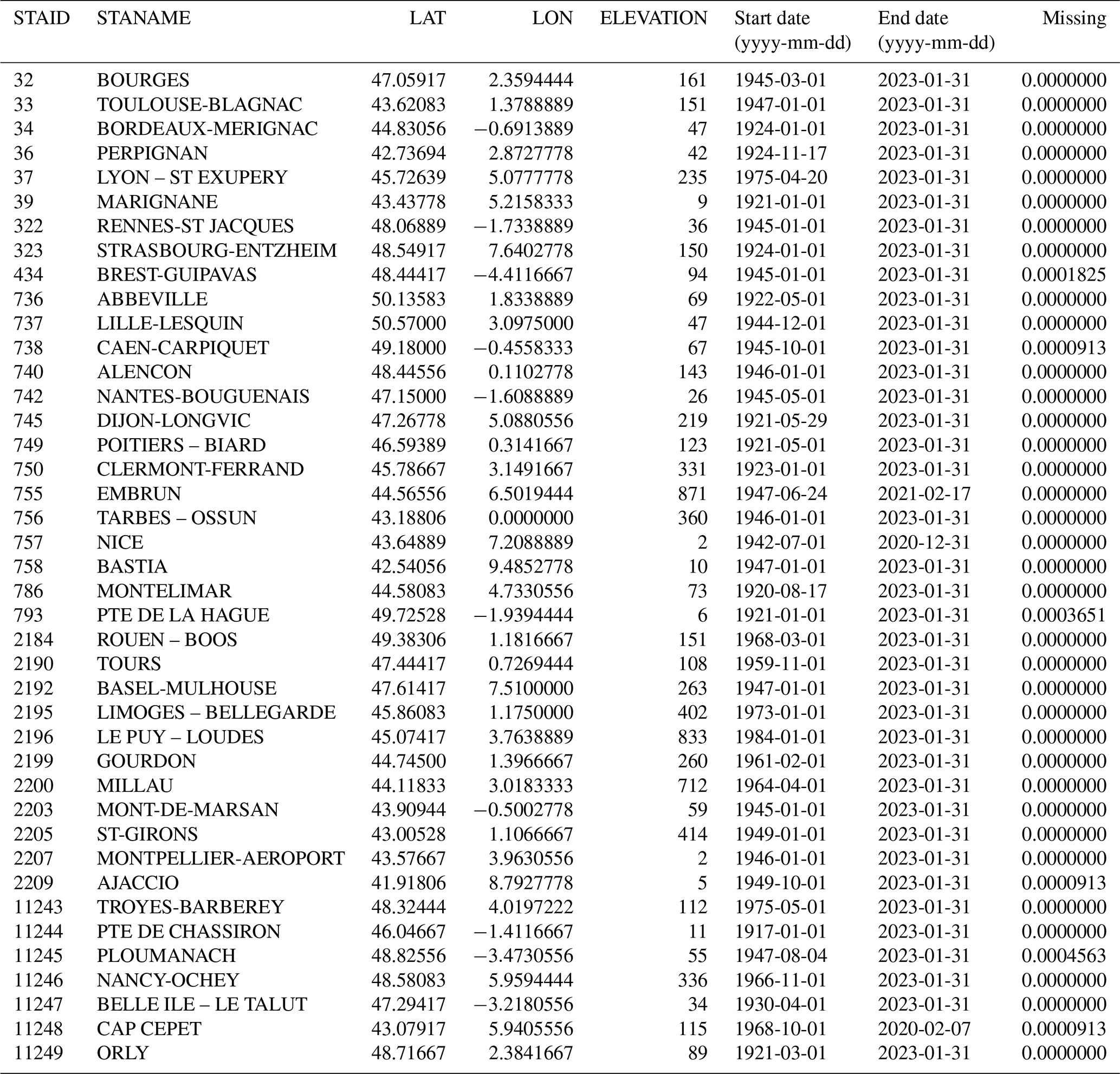
The ECA&D dataset (https://www.ecad.eu/, last access: March 2023; Klein Tank, 2002) is a high-quality European dataset of observed daily station data, covering periods that range from centuries for some stations to decades for others. We used the February 2023 version of the dataset, which includes 2068 stations across Europe with less than 8 % missing data for the period 1985–2015. From these, we selected 41 stations located in France, as shown in Fig. 1, forming the set of locations in space 𝒮_stations⊂𝒟, where 𝒟 = [6° W; 10° E] × [42° N; 52° N].

These stations are distributed regularly in space, with distances between pairs ranging from 70.95 to 1263.78 km, as illustrated in Fig. 2 (left). They are mostly situated in low-elevation areas (less than 500 m), as depicted in the histogram in Fig. 2 (right).

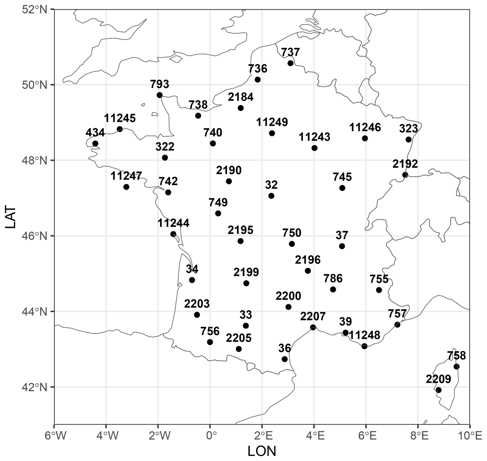
Figure 1 Selected 41 stations from the ECA&D dataset.

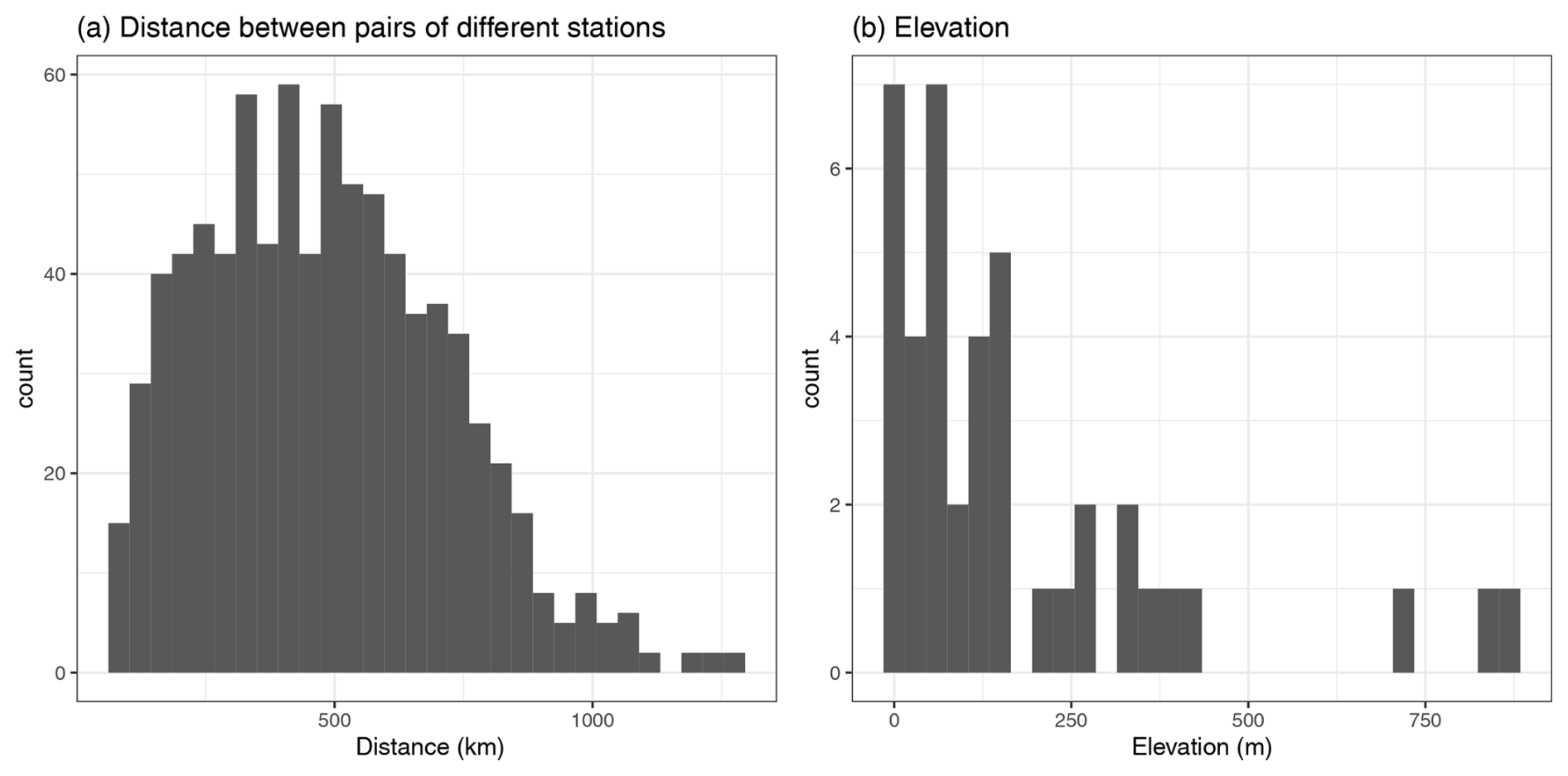
Figure 2 Histograms of the distances between stations (a) and of the elevation within the dataset (b).

For each location, missing values in the temperature series were replaced with the average value for the corresponding calendar day. As there are only few stations with missing data, and at most 6.99 % of missing values in that case, using this method does not have a significant impact on the variance of the data. Days corresponding to the 29 February were removed for simplification. The remaining data is indexed by day $t\in \mathcal{T}=\left[\right[\mathrm{1},n_T\left]\right]$, with n_T = 11 315 the number of days in the series.

2.2 The E-OBS dataset

The E-OBS dataset (Cornes et al., 2018) is a gridded version of the ECA&D dataset. It is obtained from the station data by statistical learning methods. Each day is interpolated independently first by fitting a spatial trend with a Generalised Additive Model (GAM) on the coordinates and background field, and then a kriging of the residuals with an exponential variogram and a fixed nugget parameter representing measurement uncertainty. The background field represents the monthly values of temperature. The GAM uses smoothing splines in order to model the large-scale spatial trends. The E-OBS dataset exists in 2 versions with different resolutions, 0.1 or 0.25°, we use the 0.25° version of April 2023 (version 27.0e). In the following, the set of grid points will be named 𝒮_grid⊂𝒟, with $\left|{\mathcal{S}}_{\mathrm{grid}}\right|=\mathrm{1071}$.

3 Methodology

In this section, we present the methodology for constructing a spatio-temporal model for daily average temperature. This model extends the single-site temporal model introduced by Hoang (2010) to a spatial context. We adapt the procedures for estimation, simulation, and validation to accommodate the spatio-temporal framework.

3.1 Model

Let X(s,t) be the temperature field at location s∈𝒟 and day t∈𝒯. X(s,t) is written as a combination of deterministic and stochastic terms. As in the very first weather generator of Richardson (1981), the temperature series is standardised by its variance. Following Hoang (2010), our decomposition also accounts for the annual cycle of variance and its temporal trend.

$$\begin{array}{}\text{(1)}& \begin{array}{rl}X(s,t)& =T_{\mathrm{m}}(s,t)+S_{\mathrm{m}}(s,t)\\ & +\sqrt{T_{{\mathit{\sigma }}^{\mathrm{2}}}(s,t)}\sqrt{S_{{\mathit{\sigma }}^{\mathrm{2}}}(s,t)}Z(s,t),s\in \mathcal{D},t\in \mathcal{T},\end{array}\end{array}$$

where T_m(s,t) and S_m(s,t) are the trend and the seasonality in the mean, $T_{{\mathit{\sigma }}^{\mathrm{2}}}(s,t)$ and $S_{{\mathit{\sigma }}^{\mathrm{2}}}(s,t)$ are the trend and seasonality in the variance. Z is the stochastic part called residuals. The trend terms are interpreted as representing long-term climate variations, and the seasonality terms represent the cyclic influence of the sun's radiation. Both of them represent the deterministic components of the temperature, while the stochastic part represents the intra-annual climate variability. The main assumption made in this work is that spatial and temporal non-stationarities are in the margins, while the dependence structure can be assumed stationary. Consequently, all the non stationarities are taken into account in the trend which is a function of time and space, and the dependence structure is handled in the residuals covariance which is stationary.

3.1.1 Deterministic terms

The trends in temperature over time for a given point in space s, $T_{\mathrm{m}}(s,\cdot ),T_{{\mathit{\sigma }}^{\mathrm{2}}}(s,\cdot )$ are commonly modeled using linear regression or constants. However, to better capture long-term dynamics, we prefer as in Hoang (2010) to use LOESS (LOcally Estimated Scatterplot Smoothing; Cleveland, 1979). LOESS regression fits local linear regression lines at time t to the data at time $t_{\mathrm{1}},\mathrm{\dots },t_n$ based on a chosen span parameter sp_s, with tri-cubic weighting proportional to $(\mathrm{1}-|\frac{t-t_i}{{\mathrm{sp}}_s}{|}^{\mathrm{3}}{)}^{\mathrm{3}}$. This non-parametric approach provides a more accurate representation of long-term variations compared to a simple linear trend.

The seasonality terms are modeled as trigonometric polynomials of the following form:

$$\begin{array}{}\text{(2)}& \begin{array}{rl}{S}_{\mathit{\theta }}^{\left({\mathit{\beta }}_{\mathit{\theta }}\right)}(s,t)& ={\mathit{\beta }}_{\mathit{\theta },\mathrm{1}}\left(s\right)+\sum _{i=\mathrm{1}}^{d_{\mathit{\theta }}}\left[{\mathit{\beta }}_{\mathit{\theta },\mathrm{2}i}\right(s)\cos \left({\displaystyle \frac{\mathrm{2}i\mathit{\pi }t}{\mathrm{365}}}\right)\\ & +{\mathit{\beta }}_{\mathit{\theta },\mathrm{2}i+\mathrm{1}}\left(s\right)\sin \left({\displaystyle \frac{\mathrm{2}i\mathit{\pi }t}{\mathrm{365}}}\right)],s\in \mathcal{D},t\in \mathcal{T},\end{array}\end{array}$$

with ${\mathit{\beta }}_{\mathit{\theta }}\in {\mathbb{R}}^{\mathrm{2}{d}_{\mathit{\theta }}+\mathrm{1}}$ the seasonality parameters, with θ=m or σ² either the mean or the variance, and d_θ the degree of the trigonometric polynomial. The value of d_θ has to be chosen large enough to capture seasonal details (summer, winter, transitions) but not too large to avoid overfitting.

3.1.2 A spatio-temporal model for the residuals

Due to the decomposition of Eq. (1), we assume that the spatio-temporal residuals $Z(s,t),s\in \mathcal{D},t\in \mathcal{T}$ is a Gaussian random field (Cressie and Wikle, 2015) with zero mean, stationary, and isotropic properties. Under these assumptions, the residuals are fully characterised by their covariance function

$$\begin{array}{}\text{(3)}& \begin{array}{rl}& C(h,u)=\mathrm{Cov}\left(Z\right(s+h,t+u),Z(s,t\left)\right),\\ & h\in {\mathbb{R}}^{+},u\in {\mathbb{R}}^{+},\end{array}\end{array}$$

where h is the spatial distance and u is the temporal lag.

Choosing a covariance model that reflects the properties of the data is not an easy task. There are numerous covariance models that can describe spatio-temporal dependence, see Porcu et al. (2021).

A straightforward approach to constructing a spatio-temporal covariance function is to use the product of a spatial covariance function C_S and a temporal covariance function C_T:

$$\begin{array}{}\text{(4)}& C_{\mathrm{sep}}(h,u)=C_{\mathrm{S}}\left(h\right)C_{\mathrm{T}}\left(u\right).\end{array}$$

This model is known as separable and is computationally convenient because the full covariance matrix can be expressed as the Kronecker product of two smaller matrices. However, as noted in the literature (De Iaco et al., 2019; Porcu et al., 2021), separable models may not adequately capture complex interactions between space and time, particularly for environmental or meteorological variables. In such cases, more sophisticated models that account for space-time interactions are required.

Non-separable spatio-temporal covariance functions can be constructed easily from spatial and temporal covariance functions. For instance the product-sum model is obtained using the two covariance functions C_S and C_T and positive weights $a_{\mathrm{1}},a_{\mathrm{2}},a_{\mathrm{3}}$ by constructing the spatio-temporal function $C_{\mathrm{ST}}(h,u)=a_{\mathrm{1}}{C}_{\mathrm{S}}\left(h\right)+a_{\mathrm{2}}{C}_{\mathrm{T}}\left(u\right)+a_{\mathrm{3}}{C}_{\mathrm{S}}\left(h\right)C_{\mathrm{T}}\left(u\right)$. Another construction can be made using a single covariance function C and two positive scaling factors a₁,a₂ by $C_{\mathrm{ST}}(h,u)=C\left(\sqrt{a_{\mathrm{1}}^{\mathrm{2}}{h}^{\mathrm{2}}+a_{\mathrm{2}}^{\mathrm{2}}{u}^{\mathrm{2}}}\right)$. $\sqrt{a_{\mathrm{1}}^{\mathrm{2}}{h}^{\mathrm{2}}+a_{\mathrm{2}}^{\mathrm{2}}{u}^{\mathrm{2}}}$ can be seen as a space-time distance. This construction considers time as a 3rd dimension of space, which oversimplifies the fundamentally different behaviors and units of space and time.

To tackle this problem, Gneiting (2002) proposes a construction method for classes of non-separable covariance function, that is, covariance functions that do not satisfy Eq. (4). It was extended by Allard et al. (2020) for the class of Gneiting-type covariance functions. Given ϕ a completely monotone function, γ a continuous variogram , i.e., a conditionally negative semidefinite function (Chilès and Delfiner, 2012),

$$\begin{array}{}\text{(5)}& \begin{array}{rl}& C_{\mathit{\gamma },\mathit{\varphi }}(h,u)={\displaystyle \frac{{\mathit{\sigma }}^{\mathrm{2}}}{\left(\mathit{\gamma }\right(u)+\mathrm{1})}}\mathit{\varphi }\left({\displaystyle \frac{\left|\right|h|{|}^{\mathrm{2}}}{\mathit{\gamma }\left(u\right)+\mathrm{1}}}\right),\\ & h\in {\mathbb{R}}^{\mathrm{2}},u\in \mathbb{R},\end{array}\end{array}$$

is a spatio-temporal non-separable covariance function that propose more flexibility in the interaction between the decay of spatial correlation over time than separable models. Usually, the spatial function ϕ(h) is of the form ${\mathit{\varphi }}_{\mathrm{0}}(h/r)$ with r a spatial scale parameter. In the case of Eq. (5), the space-time relationship can be considered as using a spatial scale parameter that varies with the temporal lag, with the variogram γ representing how the temporal distance interacts with the spatial distance. Another advantage of this construction is the existence of ad hoc simulation methods as described in Sect. 3.3.2.

We use the following functions for ψ, γ as in Allard et al. (2022):

$$\mathit{\varphi }\left(x\right)=\mathcal{M}(\sqrt{x};r,\mathit{\nu }),$$

where $\mathcal{M}(\cdot ,r,\mathit{\nu })$ is the Matérn function with spatial range r>0, regularity ν>0.

$$\begin{array}{rl}\mathit{\gamma }\left(t\right)& ={\left({\left({\displaystyle \frac{t}{a}}\right)}^{\mathrm{2}\mathit{\alpha }}+\mathrm{1}\right)}^b-\mathrm{1},a>\mathrm{0},b\in [\mathrm{0},\mathrm{1}],\\ & \mathit{\alpha }\in [\mathrm{0},\mathrm{1}]\end{array}$$

This leads to the model defined as:

$$\begin{array}{}\text{(6)}& C_{\mathit{\gamma },\mathit{\varphi }}(h,u)={\displaystyle \frac{{\mathit{\sigma }}^{\mathrm{2}}}{{\left({\left(\frac{u}{a}\right)}^{\mathrm{2}\mathit{\alpha }}+\mathrm{1}\right)}^b}}\mathcal{M}\left({\displaystyle \frac{h}{{\sqrt{\left({\left(\frac{u}{a}\right)}^{\mathrm{2}\mathit{\alpha }}+\mathrm{1}\right)}}^b}};r;\mathit{\nu }\right)\end{array}$$

The parameter b is called the separability parameter. When it equals to 0, the model reduces to a separable function. When b>0, the model is non-separable.

One drawback of this model is that the temporal covariance C(0,u), which describes the covariance at a fixed spatial location, can be overly constrained by the chosen parameters. A solution to this problem is to multiply Eq. (6) by a purely temporal covariance function of the form ${\left({\left(\frac{u}{a}\right)}^{\mathrm{2}\mathit{\alpha }}+\mathrm{1}\right)}^{-\mathit{\delta }}$. By introducing a slight reparametrization, $\mathit{\tau }=\mathit{\delta }+b$, this yields the Gneiting-Matern covariance model Gneiting (2002, Eq. 16)

$$\begin{array}{}\text{(7)}& \begin{array}{rl}{C}_{\mathrm{GM}}(h,u)& ={\displaystyle \frac{{\mathit{\sigma }}^{\mathrm{2}}(\mathrm{1}-{\mathit{\eta }}^{\mathrm{2}})}{{\left({\left(\frac{u}{a}\right)}^{\mathrm{2}\mathit{\alpha }}+\mathrm{1}\right)}^{\mathit{\tau }}}}\mathcal{M}\left({\displaystyle \frac{h}{{\sqrt{\left({\left(\frac{u}{a}\right)}^{\mathrm{2}\mathit{\alpha }}+\mathrm{1}\right)}}^b}};r;\mathit{\nu }\right)\\ & +{\mathit{\sigma }}^{\mathrm{2}}{\mathit{\eta }}^{\mathrm{2}}{\mathrm{1}}_{h=\mathrm{0},u=\mathrm{0}}\end{array}\end{array}$$

The nugget effect η² is added to account for small-scale variability and measurement error, as a proportion of the total variance.

This model has recently found applications and extensions, particularly for meteorological variables. Gneiting et al. (2010) introduced a multivariate spatial version of the model. Subsequently, Bourotte et al. (2016) and Allard et al. (2022) refined it by proposing multivariate spatio-temporal classes.

3.2 Estimation

Estimating the parameters of the trend and seasonality terms β_θ and the parameters ${\mathit{\sigma }}^{\mathrm{2}},{\mathit{\eta }}^{\mathrm{2}},\mathit{\alpha },a,b,r,\mathit{\delta },\mathit{\nu }$ of the covariance function simultaneously is theoretically possible maximising the whole likelihood function. However, estimating that many parameters at the same time may cause computational challenges due to identifiability issues. We prefer proceeding by a multi-stage approach and estimate “deterministic terms” first (site-by-site), introducing robustness in the estimation. This approach comes down to estimate marginal parameters first, then the covariance parameters, ensuring a stable and interpretable decomposition of the spatiotemporal structure.

3.2.1 Deterministic terms

The different components describing the temperature X(s,t) in Eq. (1) are first obtained for each station location s∈𝒮_stations, for $t\in \mathcal{T}=\left[\right[\mathrm{1}:n_T\left]\right]$ in 4 steps:

1. First, a LOESS regression on $X(s,\cdot )$ is used to get $T_{\mathrm{m}}(s,\cdot )$. The span parameter sp_s is chosen using the Modified Partitioned Cross-Validation (MPCV) of Hoang (2010).

2. The trigonometric polynomial coefficients β_m(s) (Eq. 2) involved in the seasonality of the mean $S_{\mathrm{m}}^{\left({\mathit{\beta }}_{\mathrm{m}}\right)}(s,\cdot )$, are obtained by linear regression on $X(s,\cdot )-T_{\mathrm{m}}(s,\cdot )$. The order of the polynomial d_m(s) is chosen using the Akaike criterion.

3. The variance term defined as $V(s,\cdot )={\left(X(s,\cdot )-T_{\mathrm{m}}(s,\cdot )-S_{\mathrm{m}}(s,\cdot )\right)}^{\mathrm{2}}$. $T_{{\mathit{\sigma }}^{\mathrm{2}}}(s,t)$, is obtained by LOESS regression on the variance $V(s,\cdot )$ with the same span parameter sp_s as in the trend in mean.

4. The trigonometric polynomial coefficients ${\mathit{\beta }}_{{\mathit{\sigma }}^{\mathrm{2}}}\left(s\right)$ in $S_{{\mathit{\sigma }}^{\mathrm{2}}}^{\left({\mathit{\beta }}_{{\mathit{\sigma }}^{\mathrm{2}}}\right)}(s,\cdot )$, are obtained by linear regression on $\frac{V(s,\cdot )}{T_{{\mathit{\sigma }}^{\mathrm{2}}}(s,\cdot )}$. The order of the polynomial $d_{{\mathit{\sigma }}^{\mathrm{2}}}\left(s\right)$ is also chosen with the Akaike criterion and can be different from d_m(s).

This decomposition approach is described in detail in Hoang (2010). It relies on a modified partitioned validation criterion suited to heteroscedastic and dependent data to choose the optimal smoothing parameter. The obtained residuals Z are zero-mean, stationary in time for each site s and with variance that averages to 1 over the year. The order in which the components are estimated bears some importance: if the smoothing parameter is fixed, estimating seasonality first then trends leads to the same results as estimating trends first then seasonality. However, if seasonality is identified first, it includes some part of the trend, and the optimal parameter may not be the same as the one obtained when identifying the trend first.

3.2.2 Residuals

Once the trends and seasonality components are obtained, the values of the residual field $Z(s,t{)}_{s\in {\mathcal{S}}_{\mathrm{stations}},t\in \left[\right[\mathrm{1}\mathrm{\dots },n_T\left]\right]}$ can be calculated and used to estimate the parameters of the Gneiting-Matern covariance model in Eq. (7).

The covariance matrix of the vector residuals Z is of size ${\left(\left|{\mathcal{S}}_{\mathrm{stations}}\right|\times n_T\right)}^{\mathrm{2}}$ , and computing its inverse becomes infeasible when $\left|{\mathcal{S}}_{\mathrm{stations}}\right|$ and n_T exceed a few tens, which limits the use of full likelihood methods. Composite Likelihood methods (Lindsay, 1988; Varin et al., 2011), which involve only pairwise likelihoods, are much easier to compute and exhibit good convergence properties. For a dataset $(y_{\mathrm{1}},\mathrm{\dots },y_n)$ and a vector of parameters θ, this approach means replacing the optimisation of the likelihood $L(y_{\mathrm{1}},\mathrm{\dots },y_n;\mathit{\theta })$ by the pairwise likelihood $\mathrm{PL}(y_{\mathrm{1}},\mathrm{\dots },y_n;\mathit{\theta })={\prod }_{i<j}L(y_i,y_j;\mathit{\theta })$. To further reduce the number of terms in the pairwise likelihood, we employ the Weighted Composite Likelihood (WCL), assigning a weight of 0 to pairs of sites that are far apart based on a threshold distance, chosen as half the maximum observed distance (around 650 km in this study) and a weight of 1 otherwise. This choice of half the observed distance is a usual practice in the field of geostatistics. Bourotte et al. (2016) for example have studied the relative efficiency of the pairwise likelihood estimator, showing that it first increases then decreases as a function of this cutoff parameter.

In the pairwise estimation procedure, the score function $\mathrm{\nabla }L(y_{\mathrm{1}},\mathrm{\dots },y_n;\mathit{\theta })$ is replaced by the composite score $\mathrm{\nabla }\mathrm{PL}(y_{\mathrm{1}},\mathrm{\dots },y_n;\mathit{\theta })$. In that case, the classical Fisher information matrix is no longer appropriate for variance estimation. Instead, we rely on the Godambe information matrix (Lindsay, 1988) defined as

$$\begin{array}{}\text{(8)}& \mathbf{G}\left(\mathit{\theta }\right)=\mathbf{H}\left(\mathit{\theta }{)}^{-\mathrm{1}}\mathbf{J}\right(\mathit{\theta }\left)\mathbf{H}\right(\mathit{\theta }{)}^{-\mathrm{1}},\end{array}$$

where H(θ) is the sensitivity matrix (the negative expected derivative of the pairwise score function) and J(θ) is the variability matrix (the variance of the pairwise score). Because these components are not directly available from the pairwise likelihood, they are estimated via empirical averages of the observed scores and their derivatives (Varin et al., 2011).

3.3 Simulation

Simulations are to be performed over an arbitrary set of points in space 𝒮, such as a grid of points 𝒮_grid covering the country, according to Eq. (1), where the deterministic components are extrapolated on each point, and the residuals are simulated as a spatio-temporal Gaussian field with covariance function determined by Eq. (7).

3.3.1 Spatial extension of the deterministic terms

Spatial extrapolation of parameters computed at station locations is achieved using ordinary kriging (Cressie, 1991) a statistical interpolation method that leverages spatial correlation between data points. The key to kriging is the variogram model γ(h), which quantifies the spatial dependence between points at distance h. For a spatial variable W, the variogram is defined as $\mathit{\gamma }\left(h\right)=\frac{\mathrm{1}}{\mathrm{2}}E\left[{\left(W\left(x\right)-W(x+h)\right)}^{\mathrm{2}}\right]$. Prediction at a location x₀ is a weighted sum of the observed values $W^{*}\left(x_{\mathrm{0}}\right)={\sum }_{i=\mathrm{1}}^n{\mathit{\lambda }}_{i}W\left(x_i\right)$, where the weights depend on the chosen variogram model.

Seasonality

The seasonality coefficients β_m(s),β_σ(s) for s∈𝒮 are obtained by ordinary kriging of the coefficients calculated at locations s∈𝒮_stations using a Gaussian variogram fitted to the observed data. The Gaussian variogram is defined as follows:

$$\begin{array}{}\text{(9)}& {\mathit{\gamma }}_g\left(h\right)=g_{\mathrm{1}}+g_{\mathrm{2}}\left(\mathrm{1}-\exp \left(-{\displaystyle \frac{h^{\mathrm{2}}}{g_{\mathrm{3}}^{\mathrm{2}}}}\right)\right),g_{\mathrm{1}},g_{\mathrm{2}},g_{\mathrm{3}}\ge \mathrm{0}.\end{array}$$

The annual cycles are then obtained by plugging these estimated coefficients in the seasonality functions defined in Eq. (2).

Trends

To provide the trends at each grid point, we first correct the trend in mean at sites s∈𝒮_stations using the International Standard Atmosphere (ISA) model (ISO, 1975) which describes the evolution of the standard temperature as a function of altitude:

$$\begin{array}{}\text{(10)}& T\left(z\right)=T_{\mathrm{0}}-cz,\end{array}$$

where $c=\mathrm{6.5}\times {\mathrm{10}}^{-\mathrm{3}}$ °C m⁻¹ and T₀ is the temperature at sea level (0 elevation). An equivalent temperature trend at z=0 is given by

$$\begin{array}{}\text{(11)}& T_{\mathrm{eq}}(s,t)=T_{\mathrm{m}}(s,t)+cz\left(s\right),s\in {\mathcal{S}}_{\mathrm{stations}}.\end{array}$$

T_eq is interpolated from 𝒮_stations to 𝒮 by kriging with a linear variogram ${\mathit{\gamma }}_{\mathrm{l}}\left(h\right)=g+h,g\ge \mathrm{0}$. The trend at any grid point s is then recovered by:

$$\begin{array}{}\text{(12)}& T_{\mathrm{m}}(s,t)=T_{\mathrm{eq}}(s,t)-cz\left(s\right),s\in \mathcal{S}.\end{array}$$

3.3.2 Spatio-temporal Gaussian process simulation

Simulating from the covariance function in Eq. (7) at sites 𝒮 and times t∈𝒯 means simulating from a Multivariate Gaussian process with $\left|\mathcal{S}\right|\times \left|\mathcal{T}\right|$ components. Working with large spatiotemporal grids makes it unmanageable to simulate a Gaussian process using standard procedures like the Cholesky decomposition, which has in general a complexity in $O\left(\right|\mathcal{S}{|}^{\mathrm{3}}\times \left|\mathcal{T}{|}^{\mathrm{3}}\right)$, and requires the manipulation of matrices of size $|\mathcal{S}{|}^{\mathrm{2}}\times |\mathcal{T}{|}^{\mathrm{2}}$. To address this issue, we use two different methods: an iterative method and a spectral method.

Iterative simulation

We take advantage of the temporal structure of the data, noting that time steps far apart are unlikely to be dependent. Using this observation, simulations at time t are obtained iteratively, conditioned only on the ℓ previous time steps, according to the conditional distribution of Gaussian vectors. The choice of ℓ is consistent to the temporal range parameter estimated in the covariance model. The Cholesky decomposition is then computed on matrices of size $\left(\right|\mathcal{S}|\times \mathrm{\ell }{)}^{\mathrm{2}}$ at most, which is reasonable if ℓ is not too large.

Spectral simulation

Allard et al. (2020) propose various algorithms based on spectral decomposition for simulating spatial and spatio-temporal processes with covariance models of Gneiting type, such as in Eq. (5). We use the algorithm known as the substitution approach.

Let Y be the spatio-temporal process defined by

$$\begin{array}{}\text{(13)}& \begin{array}{rl}Y(s,t)& =\sqrt{-\mathrm{2}\log \left(U\right)}\cos (\sqrt{\mathrm{2}R}\langle \mathrm{\Omega },x(s)\rangle \\ & +\left|\mathrm{\Omega }\right|/\sqrt{\mathrm{2}}W\left(t\right)+\mathrm{\Phi }),s\in \mathcal{S},t\in \mathcal{T},\end{array}\end{array}$$

where, with the notations of Eq. (5), x(s) are the cartesian coordinates of s, $U\sim \mathrm{U}\left(\right[\mathrm{0},\mathrm{1}\left]\right)$, R∼μ, $\mathrm{\Omega }\sim \mathcal{N}(\mathrm{0},I_{\mathrm{2}})$, W∼γ, $\mathrm{\Phi }\sim U\left(\right[\mathrm{0},\mathrm{2}\mathit{\pi }\left]\right)$ and the measure μ is the measure related to the Bernstein representation of ϕ. This process has the covariance function in Eq. (5). For p copies of such a process $Y_i,i\in \left[\right[\mathrm{1},\mathrm{\dots },p\left]\right]$, the Central Limit Theorem states that

$$\begin{array}{}\text{(14)}& \stackrel{\mathrm{̃}}{Z}(s,t)={\displaystyle \frac{\mathrm{1}}{\sqrt{p}}}\sum _{i=\mathrm{1}}^p{Y}_i(s,t),s\in \mathcal{S},t\in \mathcal{T},\end{array}$$

converges to a Gaussian process with the covariance function of Eq. (5) when p→∞.

This approach separates the simulation of the spatial component (simulated from μ) and the temporal component (simulated from γ), thereby reducing the dimensionality of the problem in both space and time. It is more scalable than the iterative method, which is faster for smaller grids but becomes very slow as the grid size increases. Conversely, the spectral simulation remains tractable even for larger grids, with a complexity in $O\left(p\right|\mathcal{S}|\times |\mathcal{T}\left|\right)$

3.4 Validation

To assess the validity of the weather generator, several indicators are computed for the simulations and compared to those obtained from the observations. We will compare the envelope of the simulated values with the observed values to evaluate the generator.

For spatio-temporal models, informative indicators are correlation between pairs of stations $(s_i,s_j)\in {\mathcal{S}}_{\mathrm{stations}}^{\mathrm{2}}$ both in the temperature $\mathrm{Cor}\left(X\right(s_i,\cdot ),X(s_j,\cdot \left)\right)$ and in the residuals $\mathrm{Cor}\left(Z\right(s_i,\cdot ),Z(s_j,\cdot \left)\right)$ (Sparks et al., 2018; Wilks, 1998).

Because of the non-separable assumption, it is also important to evaluate the spatio-temporal correlations, between different stations and at different time lags: $\mathrm{Cor}\left(Z\right(s_i,\cdot +\mathrm{\Delta }t),Z(s_j,\cdot \left)\right)$.

Finally, to evaluate the ability of the model to generate joint spatial extremes, we consider the pairwise conditional threshold exceedances for high (or low) quantiles, ${\stackrel{\mathrm{‾}}{p}}_{i,j}^{\mathit{\alpha }}$ (and $p_{i,j}^{\mathit{\alpha }}$): for $\mathrm{0}<\mathit{\alpha }<\mathrm{1}$ and q_α(i) such that $\mathit{\alpha }=\mathbb{P}\left(X\right(s_i,\cdot )<q_{\mathit{\alpha }}(i\left)\right)$ and a pair of stations $(s_i,s_j)\in {\mathcal{S}}_{\mathrm{stations}}^{\mathrm{2}}$

$$\begin{array}{}\text{(15)}& \begin{array}{rl}& p_{i,j}^{\mathit{\alpha }}=\mathbb{P}\left(X\right(s_i,\cdot )<q_{\mathit{\alpha }}(i\left)\right|X(s_j,\cdot )<q_{\mathit{\alpha }}\left(j\right))\text{ and }\\ & {\stackrel{\mathrm{‾}}{p}}_{i,j}^{\mathit{\alpha }}=\mathbb{P}\left(X\right(s_i,\cdot )>q_{\mathrm{1}-\mathit{\alpha }}(i\left)\right|X(s_j,\cdot )>q_{\mathrm{1}-\mathit{\alpha }}\left(j\right)),\end{array}\end{array}$$

They provide insight into how pairs of stations behave during extreme temperature events and are empirically estimated by

$$\begin{array}{}\text{(16)}& \begin{array}{rl}& {\widehat{p}}_{i,j}^{\mathit{\alpha }}={\displaystyle \frac{{\sum }_{t\in \mathcal{T}}{\mathrm{1}}_{X(s_i,t)<q_{\mathit{\alpha }}\left(i\right)\cap X(s_j,t)<q_{\mathit{\alpha }}\left(j\right)}}{{\sum }_{t\in \mathcal{T}}{\mathrm{1}}_{X(s_j,t)<q_{\mathit{\alpha }}\left(j\right)}}}\text{ and }\\ & {\stackrel{\mathrm{‾}}{\widehat{p}}}_{i,j}^{\mathit{\alpha }}={\displaystyle \frac{{\sum }_{t\in \mathcal{T}}{\mathrm{1}}_{X(s_i,t)>q_{\mathrm{1}-\mathit{\alpha }}\left(i\right)\cap X(s_j,t)>q_{\mathrm{1}-\mathit{\alpha }}\left(j\right)}}{{\sum }_{t\in \mathcal{T}}{\mathrm{1}}_{X(s_j,t)>q_{\mathrm{1}-\mathit{\alpha }}\left(j\right)}}}.\end{array}\end{array}$$

The values of ${\widehat{p}}_{i,j}^{\mathit{\alpha }}$ for the winter season and ${\stackrel{\mathrm{‾}}{\widehat{p}}}_{i,j}^{\mathit{\alpha }}$ for the summer season, for all pairs {i,j}, are then compared with the values from the simulations. Note that q_α(i) is not necessarily equal to q_α(j).

In order to better understand the capacity of the model to show spatial dynamics, let us define the quantile exceedance ratio R_α(t). It represents the proportion of locations in a set of locations 𝒮 exceeding a given quantile at any time. For t∈𝒯, $\mathrm{0}<\mathit{\alpha }<\mathrm{1}$, this proportion is written as

$$\begin{array}{}\text{(17)}& R_{\mathit{\alpha }}\left(t\right)={\displaystyle \frac{{\sum }_{s\in \mathcal{S}}{\mathrm{1}}_{X(s,t)>q_{\mathrm{1}-\mathit{\alpha }}\left(i\right)}}{\left|\mathcal{S}\right|}}.\end{array}$$

This indicator serves two main purposes. First, its survival function $\mathbb{P}\left(R_{\mathit{\alpha }}\right(t)\ge \cdot )$, computed over all time samples, describes the model's ability to generate “spatial hot days”. These are days when at least a certain (high) percentage of the domain exceeds their (high) quantile of a specified order. Second, the indicator can be used to examine the temporal evolution of this proportion, which relates to persistent heat waves. Heat waves with the most significant impact (large spatial extent over several days) are expected to exhibit a plateau for most quantiles, including even higher ones.

It is similar to the heatwave indicator of Miloshevich et al. (2023), where a measure of persistence and amplitude of anomalies is given by

$$\begin{array}{}\text{(18)}& A\left(t\right)={\displaystyle \frac{\mathrm{1}}{T}}\underset{t}{\overset{t+T}{\int }}{\displaystyle \frac{\mathrm{1}}{\mathcal{D}}}\underset{\mathcal{D}}{\int }\left(X(t^{\prime },s)-\mathbb{E}\left(X\right(t^{\prime },s\left)\right)\right)\mathrm{d}s\mathrm{d}{t}^{\prime },\end{array}$$

where T is the time scale of interest, 𝒟 the spatial domain, X the temperature. $\mathbb{E}\left(X\right(t^{\prime },s\left)\right)$ is the expected value of temperature at day t^′. This indicator averages the temperature anomaly over both space and a time period of length T. Compared to our quantile exceedance ratio of Eq. (17), it can yield non-zero values even for mild events, as long as the temperature remains above its expected value over the given period and space. However, the resulting value may be low if extreme temperatures occur only in part of the domain, while the rest of the area experiences mild or even cool temperatures, making it difficult to distinguish between different types of events. In contrast, our indicator reflects the presence of extreme values within part of the area. Additionally, this indicator is limited to detecting events that occur on a time scale close to T. Isolated hot days may go undetected.

4 Application: temperature over France

4.1 Estimated parameters

4.1.1 Deterministic components

The decomposition for each station in the ECA&D dataset is computed on the 1960–2015 data when available, or otherwise on the longest available period. Because of the initial choice of stations, it is ensured that at least the 1985–2015 period is covered. The decomposition produces the non-parametric trends and the seasonality parameters for each station.

An example of single-site decomposition is shown in Fig. 3 for the Toulouse-Blagnac station. The seasonality reveals the typical winter/summer oscillation. The trend in the mean indicates a general increase with occasional low peaks, showing an average increase of 2° over the years of observations. This highlights the necessity of including a trend and using a non-linear model. For this station, as for the others, the seasonal variance is higher in winter compared to summer. The trend in variance reflects contrasting patterns in winter and summer, along with interannual variability. The seasonality term in the variance acts as a modulating factor on the trend component, together forming the overall variance structure. The trend captures long-term changes and can be considered approximately constant throughout a single year. The seasonal component adjusts this baseline, meaning that the variance is more pronounced in winter than in summer. The slight increase in variance observed during summer in Toulouse in Fig. 3 likely reflects an increasing trend in summer compared to the annual trend, possibly because extreme events with higher amplitude tend to occur more frequently in summer in the context of French climatology. Other sites may not have this increase, instead have something like a low plateau in the summer.

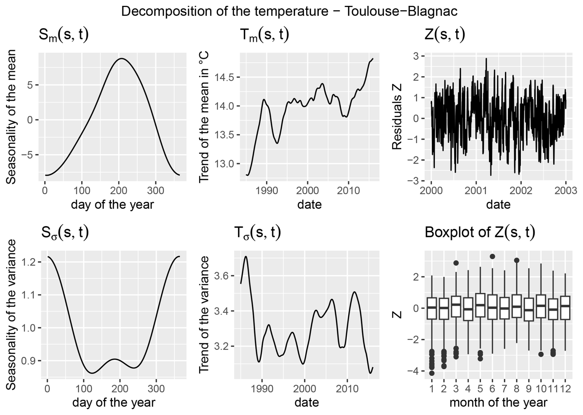
Figure 3 Decomposition at the Toulouse station (south-west of France). From left to right and top to bottom: seasonality in mean, trend in mean, 3 years of residuals Z, seasonality in variance, trend in variance and monthly boxplots of the residuals Z.

4.1.2 Spatial model

The decomposition into deterministic and stochastic terms has removed most of the seasonality from the signal. We assume hence that the model is stationary in time. However, initial investigations revealed differences between seasons in the empirical spatial covariance structure of the residuals Z. To address this, the model for the residuals is built separately for two seasons: the extended winter (October, November, December, January, February, March – ONDJFM) and the extended summer (April, May, June, July, August, September – AMJJAS). The residuals Z are assumed to be stationary in those seasons.

The estimation of covariance parameters was conducted for all years at once, for each season, by implementing the pairwise likelihood in Julia. The optimization was done using the LBFGS algorithm and automatic differentiation (AD) using an appropriate package compatible with AD for the Matérn function (Geoga et al., 2022). A maximum distance cutoff of 650 km in space and 5 d in time was applied to reduce the number of pairs and avoid rare spatial differences.

We also estimated the variance of our pairwise likelihood estimator, using the Godambe information matrix (see Varin et al., 2011). The H matrix in Eq. (8) is estimated using the Hessian of the objective function for the observations. The J matrix is estimated by computing the variance-covariance matrix of the gradient on 100 simulations.

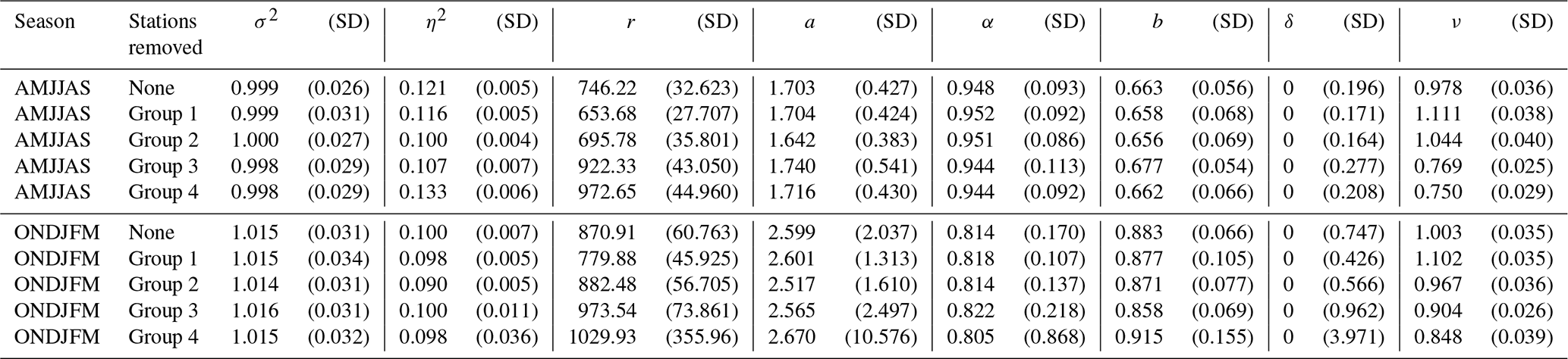
To check the robustness of the parameter estimation, the training data is split into 4 groups of equal size, with each group removed once from the estimation stage to construct 4 models in addition to the complete model estimated using all available station data. This provides insight on the impact of different input data on the estimation and simulations. The obtained parameters are shown in Table 1. Except for the spatial range parameter r, there are not many differences between estimations using the full data or estimations removing a fourth of the data.

Table 1 Estimated covariance parameters and their estimated standard deviation using a bootstrapped Godambe information matrix.

Several strategies for estimation were conducted by fixing different sets of parameters to better understand their relationships, the likelihood, and the corresponding covariance function.

The first thing to notice is that adding the flexibility in the temporal covariance with the parameter δ was in the end not necessary. In practice, the best value for this parameter is 0. As this is the minimum allowed value, estimating the hessian and gradient is not relevant and the estimated standard deviation for this parameter is not meaningful.

The spatial shape parameter ν is estimated close to 1 in both seasons, meaning the spatial regularity is not very different in the two seasons. It is interesting to see that the Matérn model for ν=1 corresponds to a linear × exponential covariance model, which is coherent with the observed empirical curves. The fact that ν is close between the seasons allows the comparison of the spatial scale parameter r, related to the typical correlation distance. It is estimated at around 800 km for both seasons, though higher in the winter than in the summer. In a Matérn model with ν≃1, the correlation drops below 0.05 at around h=5.6r. In our case, this means that for u=0 the stations become uncorrelated for a distance of more than 4000 km, which is quite large, but expected as the temperature variable exhibits strong large-scale correlation. The estimated spatial scale is inherently dependent on the data used to estimate it. When removing a fourth of the stations from the dataset, the estimated r can be quite increased in some cases, however when that happens, the summer and winter values stay coherent.

The temporal scale parameter a is estimated as higher in the winter than in the summer, but the associated standard deviation of the estimate is also quite larger. This highlights the difficulty to fit a model in the winter, where the data has both large-scale episodes and sudden variations.

The separability parameter $b\in [\mathrm{0},\mathrm{1}]$ is estimated as 0.663 in the summer and 0.883 in the winter. Both of these values are far from 0 and indicate a clear non-separable behaviour of the spatio-temporal dependence.

The obtained variogram functions $\mathrm{\Gamma }(h,u)=\frac{\mathrm{1}}{\mathrm{2}}\mathrm{Var}\left[Z\right(s,t)-Z(s+h,t+u\left)\right]$, along with the empirical function computed on the observed data $\widehat{\mathrm{\Gamma }}(h,u)$, are shown in Fig. 4. The Gneiting-Matérn model fits the data better than the separable model, which struggles to represent space-time interactions even for small time differences. The nugget effect accounts for approximately 10 % of the total variability and reflects short-range variation caused by several factors, including measurement error, micro-topographic features, and spatial variability at scales smaller than the sampling resolution.

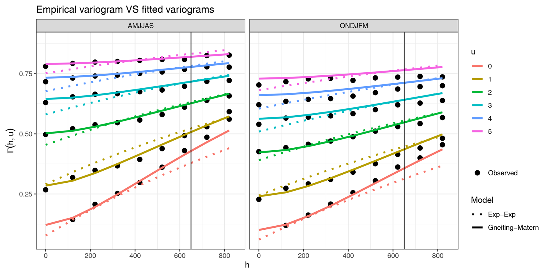
Figure 4 Variogram functions corresponding to the fitted parameter in winter (ONDJFM) and in summer (AMJJAS) for the separable model (Exp-Exp) and the Gneiting-Matérn model (Gneiting-Matern). The x-axis represents the distance in space, the y-axis holds the values of the variogram for several values of temporal distances u denoted each by a colored curve. The empirical variogram in the data is represented by the circle points. The vertical line indicates the spatial cutoff, beyond which the pairs were not taken into account in estimation. The value for $h=u=\mathrm{0}$ is missing from the empirical values because it should be the value of the nugget effect and cannot be computed in the empirical variogram.

4.2 Simulation at the training sites

Temperature series were simulated 100 times at each of the 41 fitting data points by first simulating residuals over 31 summers and 31 winters from the fitted spatio-temporal covariance model (Eq. 7) and then adding the deterministic parts in Eq. (1).

For the stochastic component, different simulation methods were employed. The Gneiting-Matérn model was simulated using both the iterative and spectral methods. Additionally, the iterative method was applied to simulate from two alternative models: first, a purely temporal version of the covariance model (no spatial component), aimed at assessing how much spatial information is conveyed by the deterministic trend and seasonality versus the spatial model in the stochastic component. A separable exponential model was also used to demonstrate the limitations of an overly simplified model.

4.2.1 An example of simulation

An example of 4 consecutive days in one simulation is presented in Fig. 5. The first column displays the observations, the second column shows a simulation based on a separable spatio-temporal covariance model, and the next two columns present simulations generated using the non-separable covariance function (via the iterative and spectral methods, respectively). The last column illustrates a simulation according to a spatially independent model. While a direct comparison of the values is not meaningful, we can evaluate whether the range of values is reasonable and whether the spatial pattern is adequately reproduced. Obviously, the last column shows a more discontinuous pattern compared to the others, highlighting the importance of incorporating a spatial component in the model.

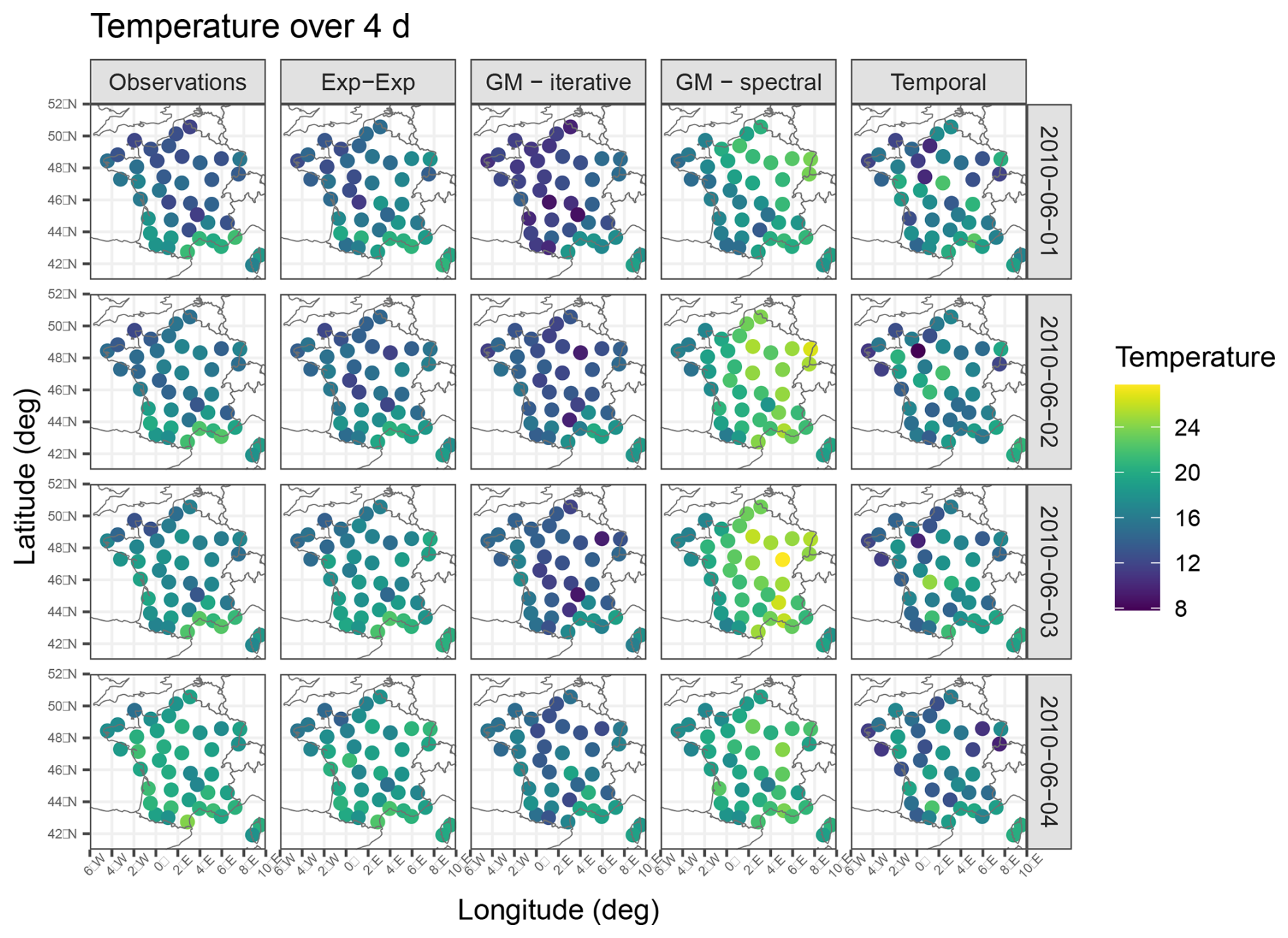
Figure 5 Observations and simulations using the separable model (Exp-Exp), the 10 d-memory simulation algorithm (GM-iterative), the spectral method (GM-spectral) and the purely temporal model (Temporal).

4.2.2 Marginal properties

Figure 6 presents the violin plots of the observed and simulated temperatures at several stations for both extended seasons (summer on the top row, winter in the bottom row). Across all models and simulation methods, the distribution of simulated temperatures closely matches the distribution of observed temperatures, demonstrating the model's ability to accurately reproduce the temperature distribution.

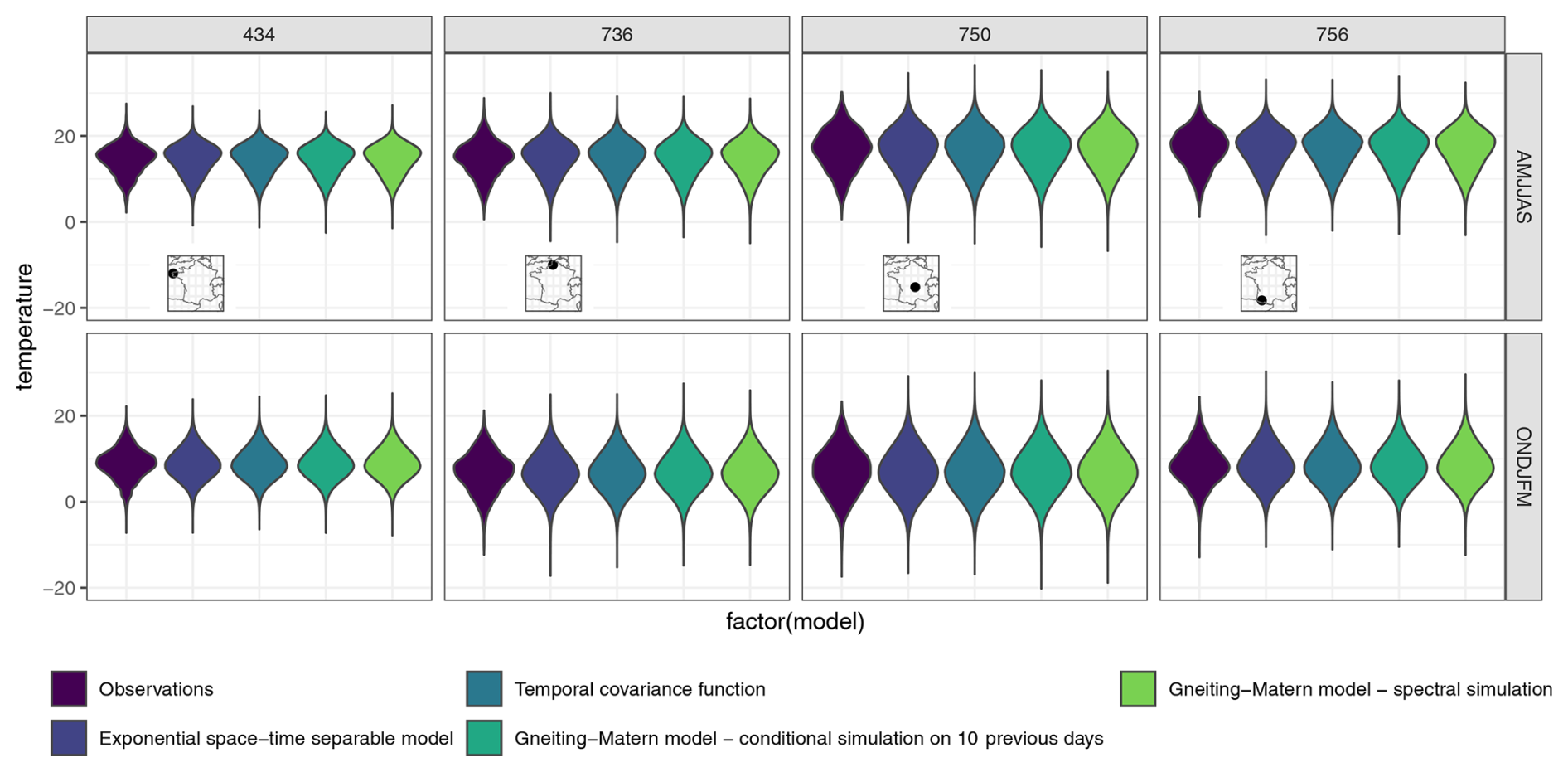
Figure 6 Violin-plot of the temperature in the two extended seasons (summer on the top row, winter in the bottom row) for 4 stations, with their corresponding locations. For simulations, 100 simulations were made using a temporal only model, a separable model and the non-separable model using the methods described in Sect. 3.3.2.

4.2.3 Spatial correlation

Figure 7 (left) illustrates the pairwise correlation coefficients between stations, comparing simulated correlation in the residuals $\mathrm{Cor}\left(Z\right(s_i,\cdot ),Z(s_j,\cdot \left)\right)$ (right) and temperatures $\mathrm{Cor}\left(X\right(s_i,\cdot ),X(s_j,\cdot \left)\right)$ (left) with their observed counterpart. For both simulation methods based on the spatio-temporal Gneiting-Matérn model – conditional simulation over the previous 10 d and spectral simulation – the observed and simulated correlations align closely with the 1 : 1 line. This indicates that this choice of correlation function effectively captures the spatial dependence structure in the data. In contrast, using a purely temporal model results in a correlation of zero for the residuals (Z). Although the corresponding simulated temperature values are non-zero due to the deterministic components, they deviate significantly from the observed values, emphasizing the benefit of incorporating a spatial model. The separable model performs similarly to the non-separable model but overestimates lower correlations. Although the significance of the non-separability property is not immediately evident in this specific graph, its advantages may become clearer when analyzing more complex spatial patterns or longer time scales.

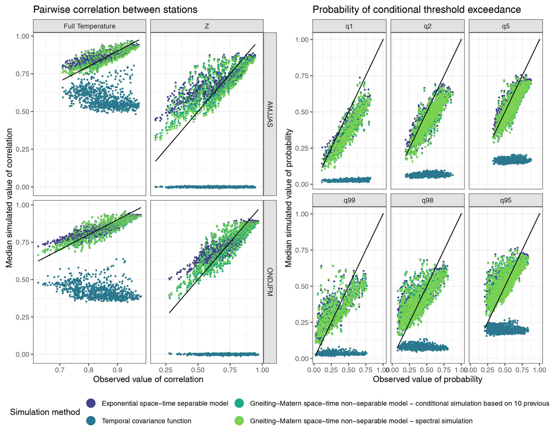
Figure 7 Correlations and conditional probabilities of threshold exceedance. x-axis: observed values, y-axis: median simulated values for 100 simulations. Left: Pairwise correlation coefficient for all pairs of stations, left in the full temperature $\mathrm{Cor}\left(X\right(s_i,\cdot ),X(s_j,\cdot \left)\right)$ and right in the residuals $\mathrm{Cor}\left(Z\right(s_i,\cdot ),Z(s_j,\cdot \left)\right)$. Top row represents the result in the extended summer, second row in the winter. Right: Empirical pairwise conditional probabilities from Eq. (15). Top: $\mathbb{P}\left(X\right(s_i,\cdot )<q_{\mathit{\alpha }}(i\left)\right|X(s_j,\cdot )<q_{\mathit{\alpha }}\left(j\right))$ for $\mathit{\alpha }=\mathrm{0.01},\mathrm{0.02},\mathrm{0.05}$. Bottom: $\mathbb{P}\left(X\right(s_i,\cdot )>q_{\mathrm{1}-\mathit{\alpha }}(i\left)\right|X(s_j,\cdot )>q_{\mathrm{1}-\mathit{\alpha }}\left(j\right))$, for $\mathit{\alpha }=\mathrm{0.01},\mathrm{0.02},\mathrm{0.05}$.

To illustrate where the non-separability property enhances the model's performance, Fig. 8 presents the covariance function C(h,u) for the residuals Z at various time lags u. This function is computed from both the observations and one simulation for each of the three models: temporal only, separable, and non-separable. The purely temporal model fails to reproduce the observed correlations, as expected. Because the observed spatial covariance is scattered, making direct comparison difficult, a LOESS smoothing line is added to help visualise the difference between the separable and non-separable models. For u=0, both spatio-temporal models (separable and non-separable) overestimate the covariance for stations that are far apart, reflecting the previous observations from pairwise correlations. However, the non-separable model demonstrates a modest improvement from the separable model in these cases. This overestimation likely results from the fact that far-apart station pairs are underrepresented in the dataset and were not used during model training. For non-zero time lags, the separable model tends to overestimate high covariances and underestimate low covariances compared to the non-separable model. This discrepancy emphasizes the necessity of using a non-separable model, as further detailed in Appendix B, where we investigate empirically the separability of the data.

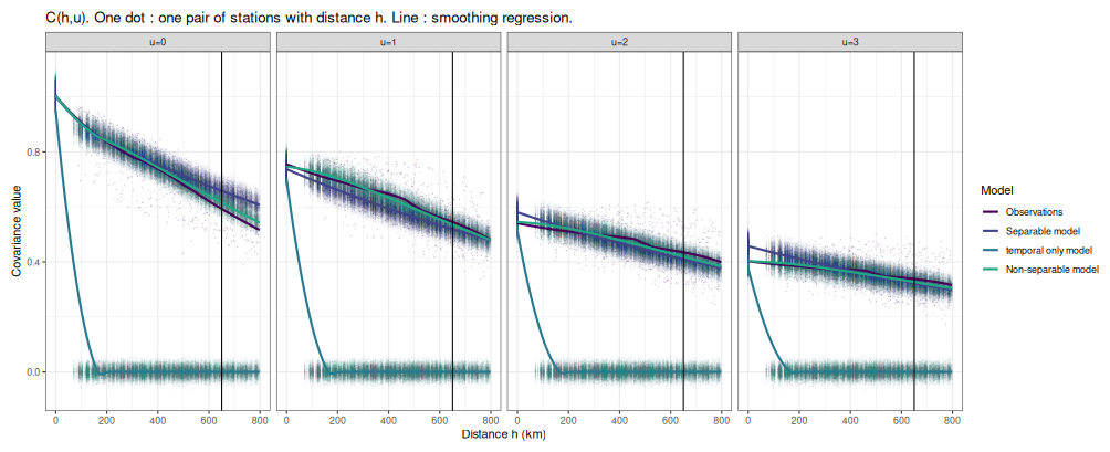
Figure 8 Empirical covariance in the reduced variable Z, C(h,u), for different time lags $u=\mathrm{0},\mathrm{1},\mathrm{2},\mathrm{3}$. Each dot denotes the covariance between a pair of stations separated by the distance h. The small dots are the covariance for each pair, the solid line the loess values. The colored dots correspond to 100 simulations for the observations and all 3 possible models: temporal-only, separable, non-separable.

Figure 7 (right) shows the pairwise conditional probabilities of threshold exceedance in the observations compared to the simulations. For all models except the spatially uncorrelated model, the values in simulation are in the range of the observations. For the highest quantile (0.99), the small probabilities are overestimated, and the large probabilities are underestimated. This means that the dependance is overestimated when it is high, and underestimated when low. Such behaviour was to be expected as the Gaussian distribution is known to be asymptotically independent (Coles, 2001). Nonetheless, once the effects of trends and seasonalities are accounted for, the resulting extremal dependence in the simulated temperatures aligns reasonably well with the observed data, except at the very most extreme quantiles. Enhancing the model accordingly would require at least two improvements. First, adopting a distribution that better captures the behavior in the extremes, such as (extended) Pareto distributions. However, this shift would introduce new complexities during parameter estimation. An alternative would be to explicitly model the extremes in a separate statistical framework. Second, choosing a dependance structure for one that exhibits stronger dependence in the extremes such as max-stable models which are asymptotically dependent or one intermediate.

4.2.4 Quantile Exceedance Ratio

Focusing on the summer months, with quantiles q_i(α) and Quantile Exceedance Ratios R_α(t) (as defined in Eq. 17) computed only on June, July and August (JJA) data and simulations, the survival function of R_α(t) for several values of α is represented in Fig. 9. There is about 10 % chance that at least 15 out of the 41 stations exceed their 90 % quantile at the same time. In the simulations, it has about 9 % chance. Overall, the simulations tend to underestimate the probability to exceed a threshold for several locations at the same time. This is coherent with the previous observations on pairwise threshold exceedance probabilities, where we found that the simulations underestimated the high values.

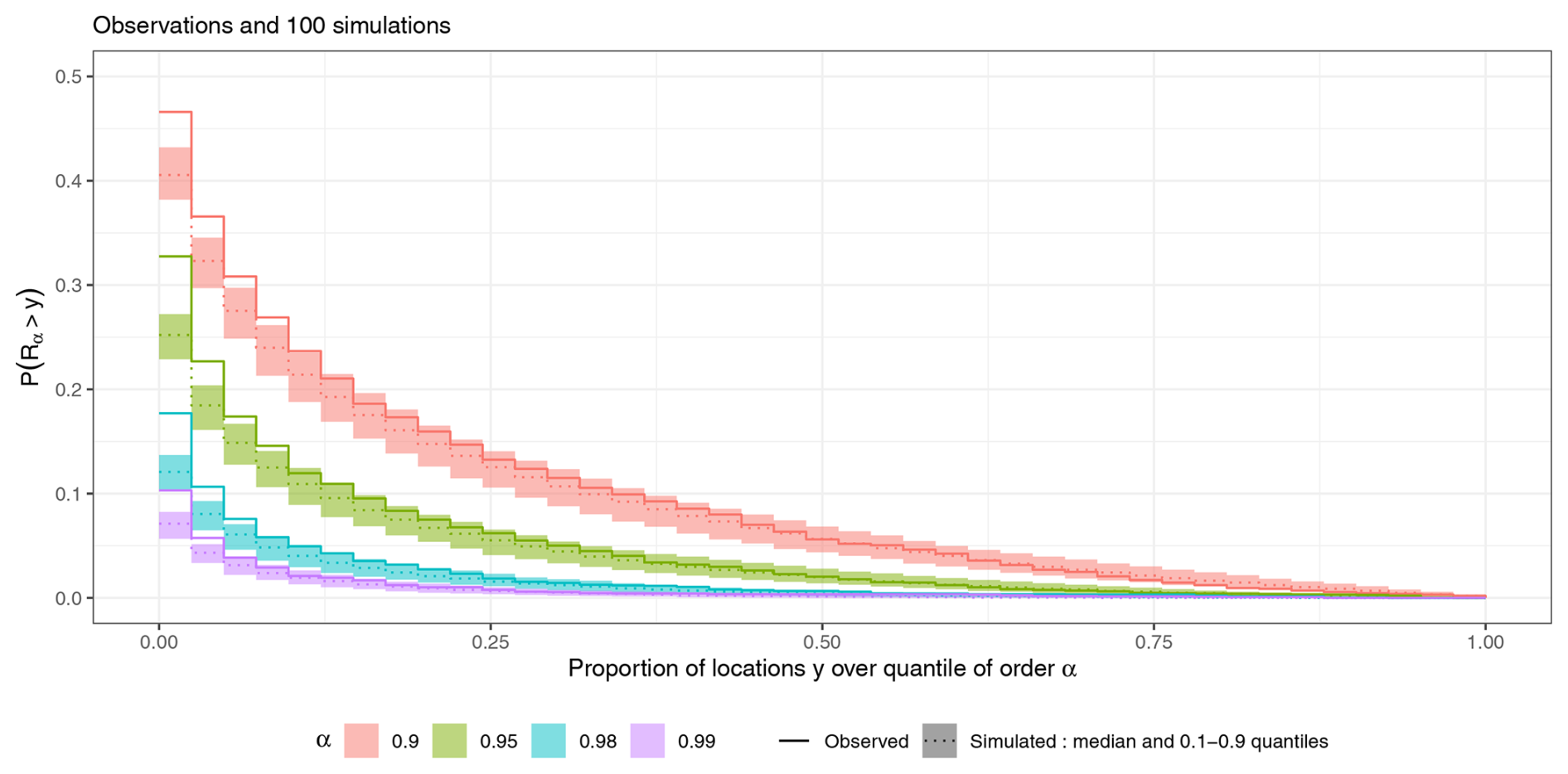
Figure 9 Survival function of the Quantile Exceedance Ratio, ℙ(R_α(t)≥y) for several quantiles α, computed on the observations (ECA&D) and simulations from the non-separable model.

4.3 Simulations on a grid

This section shows the use of the generator trained on the station data for simulation over the E-OBS grid. The simulations are then compared to the E-OBS data that serves as a reference.

4.3.1 1985–2015 simulations

We generated 100 simulations over the same 1985–2015 period. Examples of these simulations are shown in Fig. 10, alongside the corresponding values from the E-OBS database. Among the 100 simulations, we selected examples closest to the median temperature of E-OBS, as well as the coldest and warmest simulations. Although direct comparison of day-to-day values is not meaningful, the overall patterns are similar. The range of simulated temperatures is broad, accommodating both cool and hot days with strong temporal correlation.

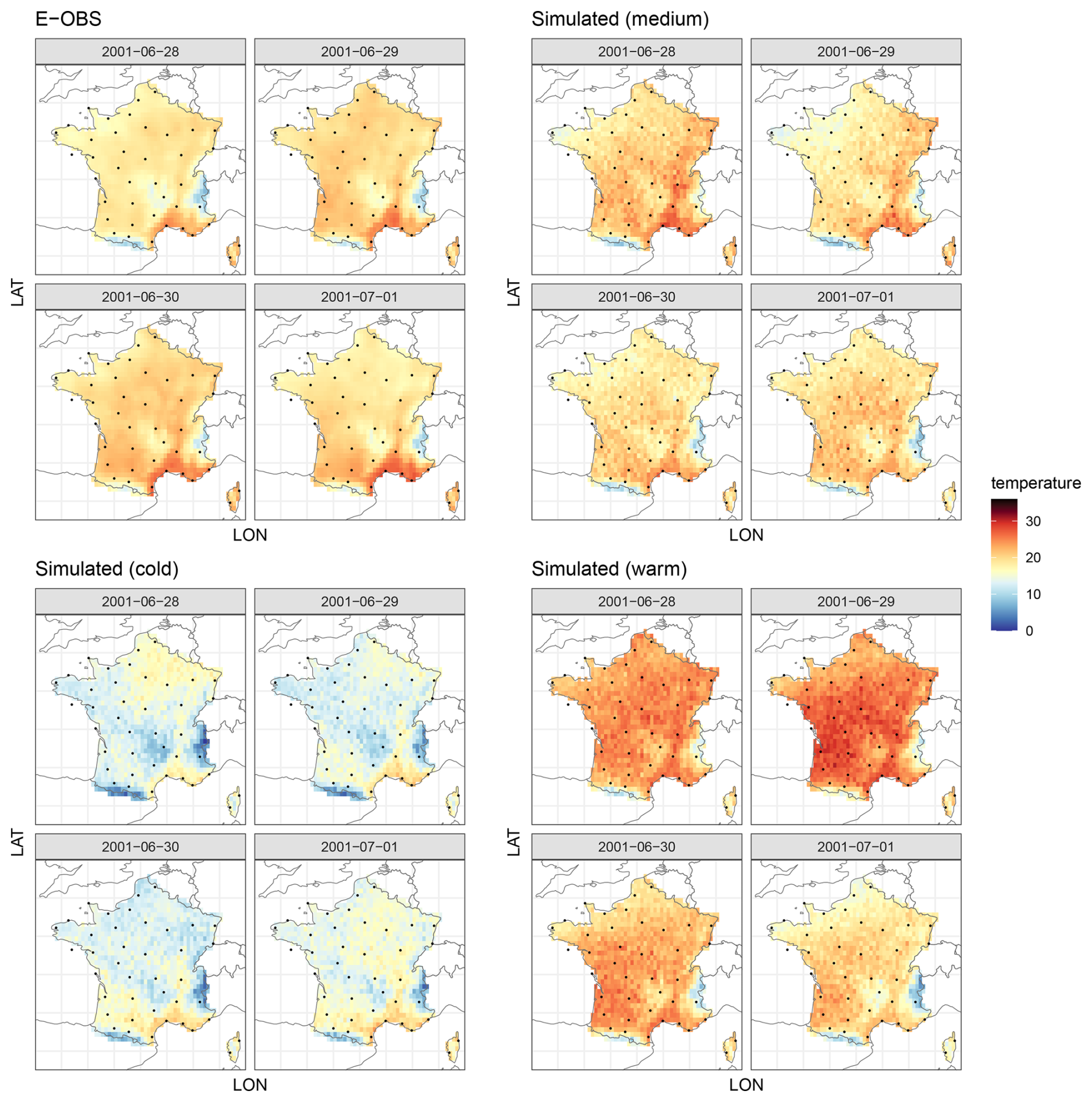
Figure 10 From left to right: 4 d in E-OBS, an example of the same simulated 4 d, coldest and warmest simulation for the same days.

The simulated temperatures appear less smooth than those from the E-OBS dataset, which is expected for several reasons. First, E-OBS is an interpolated product based on station measurements, resulting in inherently smoother spatial fields. In contrast, our simulation model includes a nugget effect, which explicitly captures short-range variability – such as measurement error or micro-scale environmental effects – as a proportion of the total variance.

The spatial resolution of E-OBS is approximately 25 km, while the minimum distance between stations in the training data was closer to 100 km. This relatively coarse station density limited the model's ability to capture very short-range spatial structure, likely leading to an overestimation of the nugget effect and, consequently, rougher simulations.

However, the presence of a nugget effect in our model is not necessarily a drawback. It reflects a realistic component of spatial variability at small scales and ensures that simulations account for local heterogeneity. With denser station coverage, this short-range behavior could be estimated more precisely, potentially yielding smoother simulated fields. Alternatively, removing the nugget effect would produce smoother outputs, but at the risk of under-representing local variability and generating unrealistically homogeneous fields.

The quantile exceedance ratio R_α(t) can be analyzed in the same manner. Figure 11 shows the survival function for various quantiles. These quantiles are extracted from the E-OBS database for each grid cell. The simulated survival function is represented by a ribbon spanning the 0.1–0.9 quantile range of the simulations, with a dotted line indicating the median value, and the survival function in E-OBS is represented by a full line. The simulations tend to overestimate the number of heat days over smaller areas while underestimating the frequency of events covering larger areas, compared to the observed values.

Figure 11 Survival function ℙ(R_α(t)≥y) for several quantiles α, computed on E-OBS and gridded simulations.

It is also important to reproduce not only isolated hot days but also sequences of hot days with length comparable to the observed events. Figure 12 illustrates the evolution of R_α(t) for several quantiles in some observed summers and some simulated summers. It illustrates the model's ability to reproduce summer heatwave characteristics in terms of duration, intensity, and spatial extent. Each panel shows the proportion of the domain exceeding a temperature quantile (color-coded) over the days of summer. The two left panels show observed summers of 2003 and 2009, with 2003 notable for its intense and long-lasting heatwave affecting much of France, used here as a reference. Its exceptional spatial extent and duration are highlighted with arrows. The other panels show examples of simulated summers. These demonstrate the model's capacity to generate heat events of varying types: short and localised events (all graphs), short events that are large in space (bottom right), events resembling the 2003 heatwave in both intensity and duration (top middle and top right), and even a long-duration heatwave with slightly less intensity than 2003 (bottom middle). These examples support the model’s ability to capture realistic variability in heatwave behavior.

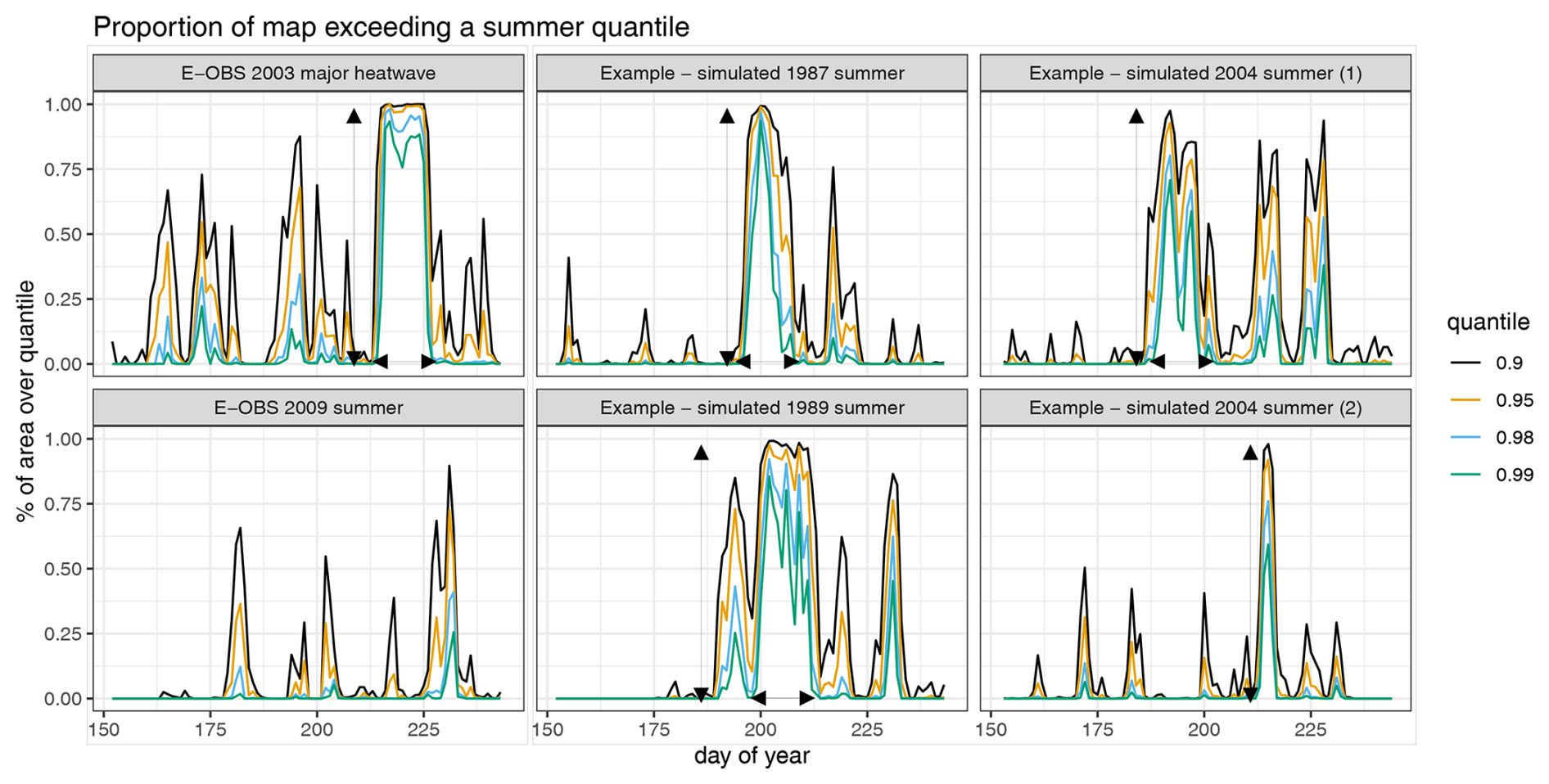
Figure 12 Spatial coverage of extreme heat over time, R_α(t), for several quantiles α, across two observed summers and four simulated ones.

We consider spatial heat episodes as sequences of days when the temperature exceeds a specified threshold in at least a given proportion of the domain. Figure 13 shows the distribution of heat episode lengths for both E-OBS (red dots) and the 100 simulations (black bars).

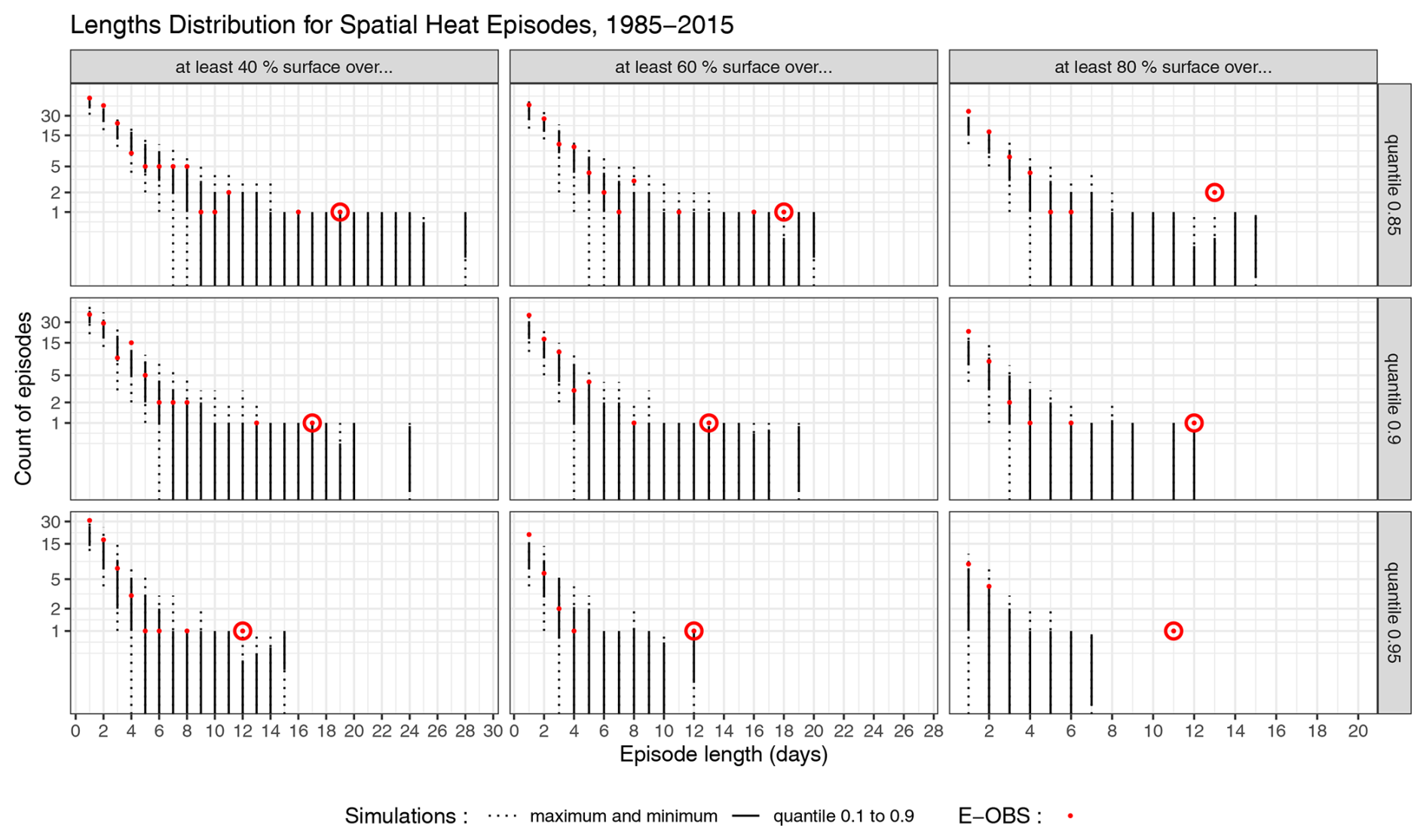
Figure 13 Length distribution of heat events for the observations and for 100 simulations. From left to right : spatial size of event (cumulative % of surface over the quantile threshold), from top to bottom: 0.85,0.9, and 0.95 quantile. For each plot, the x-axis represents the episode length and the y-axis holds the number of events of this length in one 1985–2015 series. Log-scale on the y-axis. The dotted bars indicate the whole range of values found in the simulations, while the full bars represent the 0.1–0.9 quantile range of simulated values. The red dots indicate the E-OBS values, the circled dots represent the 2003 heatwave.

For heat episodes that cover at least 40 % or 60 % of the domain, and for moderate temperature quantiles such as the 0.85 or 0.9 quantiles, the observed values fall within the range of simulated values. The model even succeeds in generating events longer than those observed. However, for higher spatial proportions, the simulations struggle more to generate extended episodes, indicating some limitations in replicating the most extreme spatial heat events. This is coherent with the conclusion given by the previous Fig. 11.

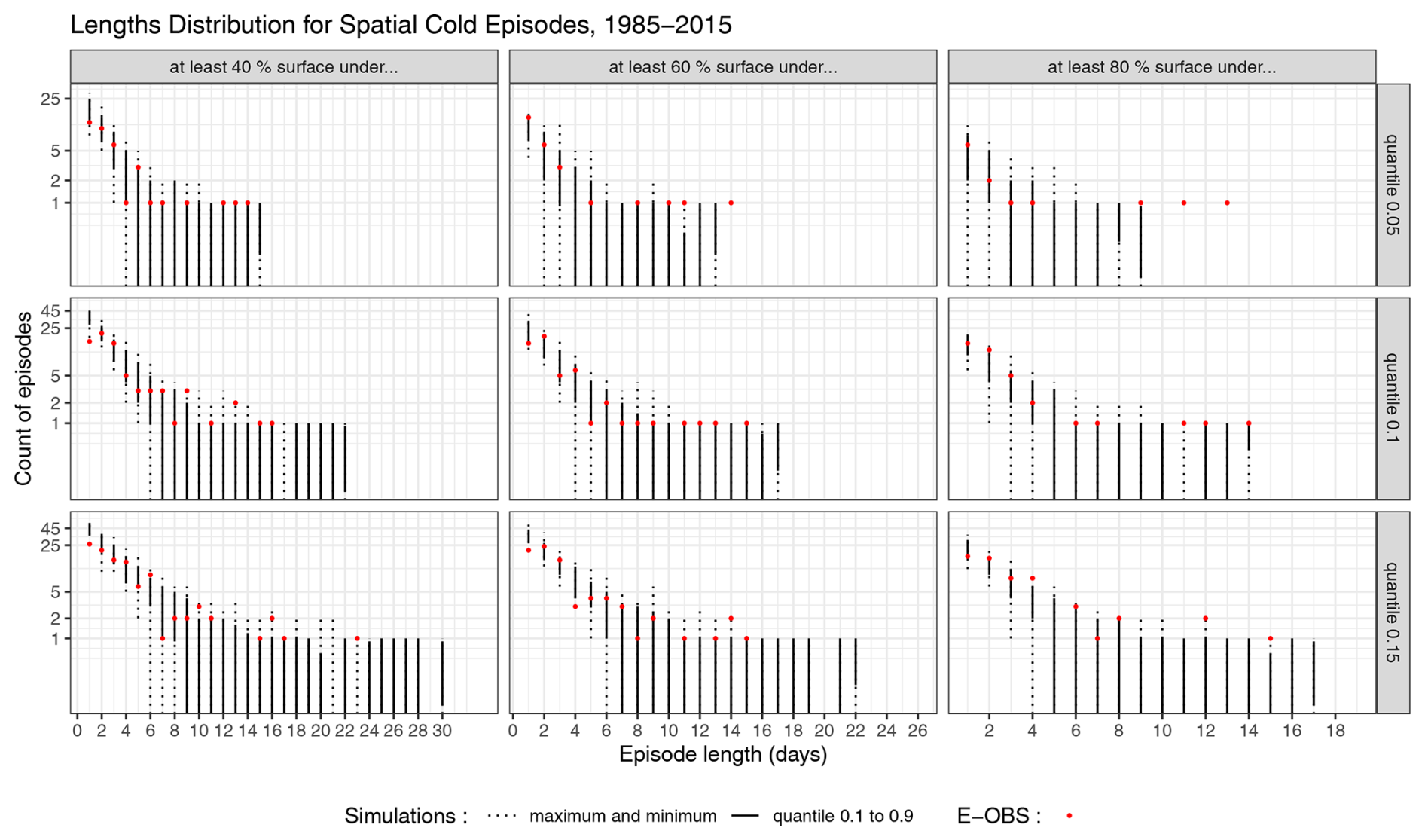
Figure 14 Distribution of the length of cold events in the observations and in 100 simulations. From left to right: spatial size of event (cumulative % of surface over the quantile threshold), from top to bottom: considered quantile. For each plot, the x-axis represent the episode length and the y-axis holds the number of events of this length in one 1985–2015 series. Log-scale on the y-axis. The dotted bars indicate the whole range of values found in the simulations, while the full bars represent the 0.1–0.9 quantile range of simulated values. The red dots indicate the E-OBS values.

Cold events can be similarly defined as sequences of days when the temperature in winter (December–January–February) is under a given threshold for a given proportion of the domain. Figure 14 shows the distribution of the length of cold events in the observations and the simulations. For events that are below the 0.05 quantile, the model generates an appropriate number of single-day events for all considered spatial extents, but does not reproduce events with high temporal length. However, for such a low quantile and for a large spatial extent, the observations contain only a few events. For milder quantiles, the model is able to generate longer events but overestimates the number of single day events.

Using the E-OBS observational database as a reference, we analyze the model’s ability to replicate heat and cold events, defined by the exceedance of specific temperature quantiles over large spatial areas. The model captures the overall behavior of temperature extremes, including heatwave sequences similar to the notable 2003 European heatwave. However, while it successfully reproduces the frequency and duration of moderate heat episodes, the model tends to overestimate the occurrence of heat events in smaller regions and underestimates those covering larger areas. For cold episodes, the model generates realistic short-term events but struggles to reproduce longer events, particularly those covering large spatial extents.

4.3.2 Projections for 2016–2023

In this section, we demonstrate how the complete model can be utilised for near future projections. The following reasonable assumptions are made:

• The seasonality in mean and variance will remain the same in the near future. This is because they are estimated mainly as the result of the incoming solar radiation linked to earth rotation. The temperature change over time is included in the trend part which is removed first.

• The spatio-temporal dependence in the residuals Z will remain unchanged in the future, as far as only the near future is considered.

• Future trends in mean and variance have been derived here from the observations, but can be obtained from climate projections using various scenarios if farther future periods are targeted.

• Should the projections concern farther future periods, the seasonality in mean and variance and the spatio-temporal structure of the residuals may have to be fitted again on climate projections.

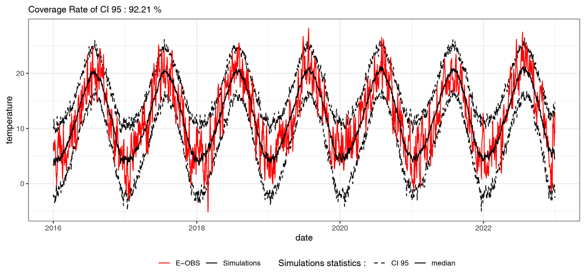
Figure 15 Mean temperature over the France grid for 2016–2022. The 100 simulations are obtained using a model fitted on the 1985–2015 period. Observed temperatures are shown in red. Simulations are represented with dotted black lines for the quantiles of order 0.025 and 0.975 of the simulated temperatures, and a solid black line for the median simulated temperature.

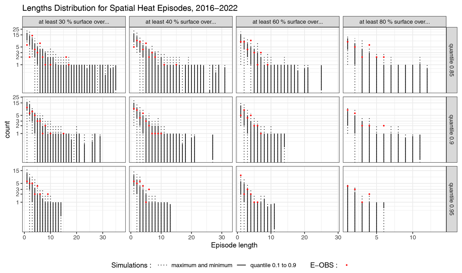
Figure 16 Distribution of the length of heat events in the observations (red dots) and in 100 simulations (black bars), for the period 2016–2022.

The stochastic model is calibrated using data from 1985 to 2015. To validate the model's projection capabilities, we apply it to the period from 2016 to 2022. Trends in mean and variance for this future period can be derived using the same decomposition method, but with updated data from 1985 to 2022, while retaining the seasonal patterns from the earlier period.

We generated 100 simulations based on the updated trends and previous seasonality and stochastic models. The resulting mean temperatures averaged across the France grid are illustrated in Fig. 15 by their medians and 95 % intervals, and compared with the E-OBS values. The coverage rate of the interval is 92.21 %, which is close to the expected 95 %, with a small underestimation of the real variability. This demonstrates the model's capability to accurately project future temperatures, provided that the trends are known. This shows that future climate projected trends can be plugged into the model if farther future is considered.

The year 2022 experienced many important heatwaves. In Fig. 16, the distribution of the length of spatial heat episodes are represented for different spatial thresholds. The quantiles used to define the “hot days” are the 1985–2015 quantiles.

Most observed episodes fall within the range of the simulations. For all considered quantiles and spatial extents, the model successfully generates heat episodes that are longer than those observed. This suggests that the model can account for the possibility of longer heat waves than those recorded.

5 Conclusions

The spatio-temporal stochastic weather generator presented in this study and applied to French station data is a tool to generate realistic temperature series across a large area. By leveraging spatial statistics, the model effectively captures spatial-temporal correlations, enabling the simulation of plausible large-scale temperature events across the study area. This capability is particularly valuable for applications requiring temperature modeling across various locations, whether data is available for specific points, and even when those points are spread out spatially. To our knowledge, previous studies using spatial statistics have focused on more localised regions and have not addressed temperature trends with the same level of precision.

To study a changing climate, the trend components of the model can be adjusted based on climate simulation outputs and various scenarios. By either keeping the seasonal cycles and spatial covariance structure stationary, or retraining them based on corrected model output, this approach allows for generating numerous simulations corresponding to different scenarios or specific areas of interest. This method significantly reduces computation time compared to physical models, thereby complementing physical simulations and providing valuable insights into future climate conditions.

Further investigation into the marginal distributions may be necessary to improve the representation of extreme conditions, such as extreme heat events. For many applications, accurately sampling these unfavorable conditions is crucial. Some further investigation on the margins may also be needed. For instance, the skewed-exponential-power distribution used in Evin et al. (2019) could provide a better fit for the temperature distribution, especially in the tails.

In this paper, while the Gaussian model was used, and although it is known to lack extremal dependence, the spatial extremes were found to be reasonably well represented in the simulations. However, there was a slight underestimation of the high-temperature extremal pairwise correlations. Future research should explore different non-Gaussian dependence structures, as the Gaussian approach, while adequate for temperature alone, might not be suitable for other variables or for modeling cross-correlations.

Additionally, there are plans to extend this model to cover the entire European continent. This expansion may require addressing issues of non-stationarity due to varying climates across different regions.

Many applications require modeling additional variables such as precipitation, wind speed, or solar radiation, which necessitates accounting for their spatial and temporal cross-correlations. While the Gneiting-Matérn model used in this study is well-suited for temperature, extending it to multiple variables presents challenges. Authors such as Bourotte et al. (2016) and Allard et al. (2022) have proposed flexible multivariate covariance functions that extend the univariate Gneiting-Matérn class. However, these models have not been tested over large areas like ours and may not be fully suitable. As for the marginals, they cannot be considered Gaussian. For precipitation amounts, while mixtures of Gamma or Exponential distributions are commonly used, they may not always adequately capture the right tail of the distribution. The Extended Pareto distribution, as proposed by Naveau et al. (2016), could be a valuable alternative, as it is designed to model both the bulk and the tail of the distribution effectively.

Another approach involves incorporating weather types into the model. Weather type modeling breaks down the dependence into different types of days, allowing for simpler models to be applied to each type (Allard et al., 2015; Stoner and Economou, 2020; Dawkins et al., 2022; Gobet et al., 2025). The sequence of weather types can be modeled using a Markov chain. Weather types can be learned from the data, with the simplest classification being dry/wet states, while more complex models might include hidden or unobserved states. Future work will build on the extensive literature on multi-site and spatial weather type models to integrate the temperature generator from this study into a comprehensive multivariate generator.

Appendix A: Data locations

The Table A1 presents the stations used in this study: station identifier STAID, name STANAME, coordinates in the LON/LAT format and elevation. Additionnal columns hold the start and end date of the temperature file, and the column “missing” holds the proportion of missing data over the period 1985–2015.

Table A1 List of the French ECA&D stations.

Appendix B: Separability

The choice of covariance structure reflects the non-separability in the data.

The separability property holds if the covariance function of the process under study satisfies

$$\begin{array}{}\text{(B1)}& C(h,u)=C(h,\mathrm{0})C(\mathrm{0},u)\end{array}$$

where $C(h,\mathrm{0})=C_{\mathrm{S}}\left(h\right)$ is the covariance in space and $C(\mathrm{0},u)=C_{\mathrm{T}}\left(u\right)$ is the covariance in time.

Tests have been proposed to study this assumption such as in Li et al. (2007), but they fail in practice with our temperature data because of the strong correlation in time. However, it can be empirically seen in Fig. B1 that for most considered $h,u\in [\mathrm{1},\mathrm{\dots },T]\times \mathcal{D}$, $C(h,u)\ge C(h,\mathrm{0})C(\mathrm{0},u)$. This means that not only is the covariance of the data non-separable, but also that according to the definition of De Iaco and Posa (2013), the non-separability is said to be “positive”.

Conveniently, any model of the Gneiting class satisfy this property, which is why this class was chosen.

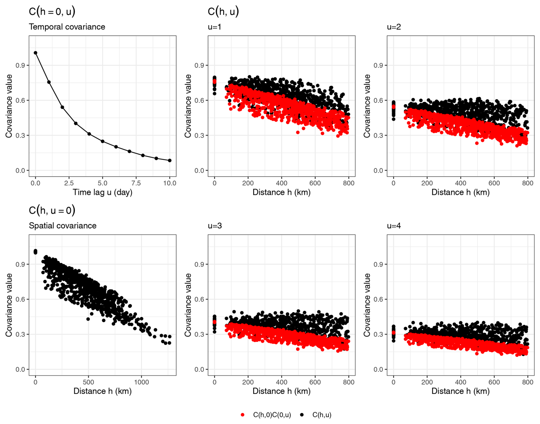
Figure B1 Comparison between the empirical spatial-temporal covariance function (black) and the product between the spatial and temporal covariance function (red). Each dot denotes the covariance between a pair of stations separated by a distance h.

Appendix C: Parameter estimates using station data

C1 Gridded trends

The Fig. C1 shows the interpolated temperature trend using the equivalent temperature that takes into account the elevation, compared to trends obtained from the much more complete E-OBS database. The addition of geographical information seems to correct quite well the values of the trend in mean.

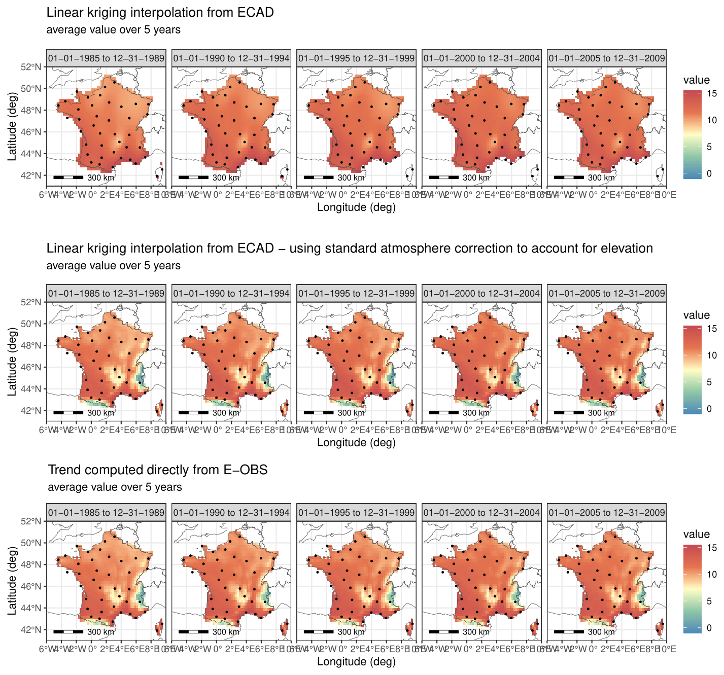
Figure C1 Trend in mean interpolated from site-by-site decomposition using ordinary kriging and altitude equivalent temperature, compared with trends obtained directly from the E-OBS database.

Figure C2 shows the average maps over 5 years of the standard deviation trend, using the kriging method. The stations are indicated by dots. The variance is stable in mean over 5 years.

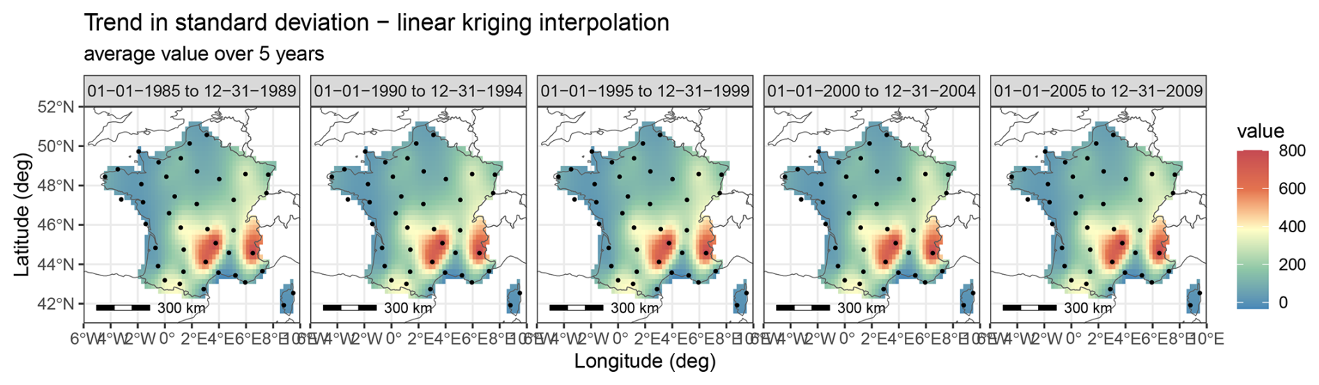
Figure C2 Trend in standard deviation, interpolated from site-by-site decomposition using ordinary kriging.

C2 Gridded seasonality coefficients

Kriging with a Gaussian variogram model was used to interpolate each seasonality coefficient. Resulting coefficients maps are given in Figs. C3, C4. Similar to what is observed when working with the trends, removing stations from the training set sometimes introduced significant error. It is mostly the case when several stations from the borders of the domain are missing, or in the case of the mountainous stations pointed out previously.

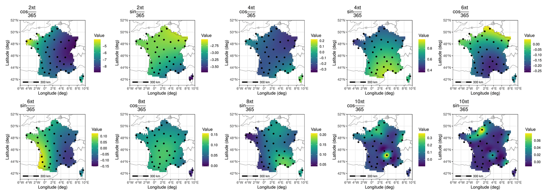
Figure C3 Seasonality coefficient for the mean, interpolated from site-by-site decomposition using ordinary kriging.

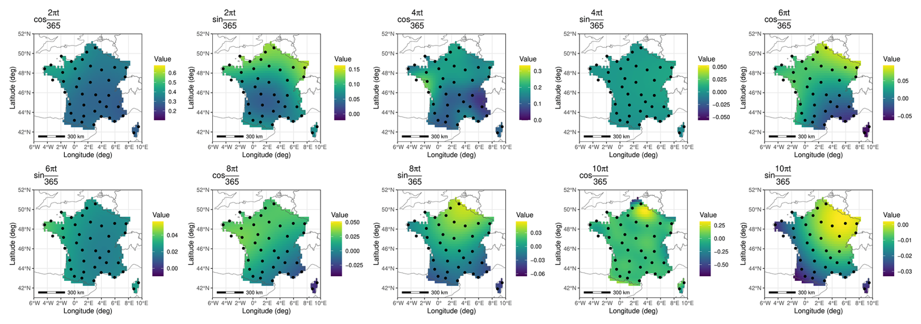
Figure C4 Seasonality coefficient for the standard deviation interpolated from site-by-site decomposition using ordinary kriging.