Bayesian hierarchical modelling of intensity-duration-frequency curves using a climate model large ensemble

Accurate modelling of extreme precipitation is vital for predicting future risks and informing adaptation strategies. Here, we compare and evaluate six different extreme value statistical models for hourly to 48 h extreme precipitation in southern Germany, with a primary focus on duration-dependent Generalized Extreme Value (dGEV) distributions. To assess model performance, particularly in capturing tail behavior, we utilize the 50-member single model initial-condition large ensemble of the Canadian Regional Climate Model version 5 for the period 1980–2019. The large sample size of 2000 simulated years enables a robust sampling of extreme quantiles. Using a sub-sampling strategy with 30 to 100 years, we compare the efficacy of Bayesian methodology, in particular Bayesian hierarchical models, against frequentist models (L-moments and Maximum Likelihood Estimation – MLE) in representing the tail risk of 100-year return levels based on limited sample sizes. Hierarchical models allow us to give special emphasis on the dimensionality of the GEV shape parameter, a critical factor for tail behavior. Our findings reveal that a shape parameter varying over durations but fixed across space is beneficial for the prediction of the 100-year return level. The resulting Intensity-Duration-Frequency (IDF) curve shows the highest accuracy and smallest confidence intervals proving its robustness. Compared to the standard GEV estimated by L-moments, our proposed model can reduce the relative error of the 100-year return level from 18.1  % to 8.8  % based on a 30-year sample size. Furthermore, our analysis reveals fundamental limitations of the Anderson-Darling test for extreme value model selection, demonstrating its poor correlation with predictive skill for upper quantiles – a critical finding for climate risk applications.

1 Introduction

Extreme precipitation can severely impact various sectors such as infrastructure design, water resource management and agriculture (Yang et al., 2020; Mattingly et al., 2017; Schwarzak et al., 2015). Thus, different rainfall durations can trigger a variety of impacts. Short intense duration precipitation is commonly associated with convection and can lead to urban flooding, flash floods (often steep catchments), Hortonian overland flow, and riverine floods in small catchments (Haslinger et al., 2025; Fereshtehpour and Najafi, 2025; Ruiz-Villanueva et al., 2012; Fowler et al., 2021). Long persistent precipitation is mainly associated with synoptic-scale meteorological systems, such as frontal or orographic systems, leading to riverine floods in larger catchments, often caused by saturation overland flow (Tarasova et al., 2019). This impact will increase in the future with increasing frequency and intensity of extreme rainfall events in a warmer climate (Fischer et al., 2021; Seneviratne et al., 2022; Poschlod and Ludwig, 2021). Computing the magnitude and probability of extreme events through statistical models, can help us assess risks of extremes from climate-related disasters (Ghil et al., 2011; Naveau et al., 2020).

Extreme rainfall is often modeled using the Extreme Value Theory (EVT), which focuses on the tails of distributions (Fisher and Tippett, 1928). Sampling maximum precipitation values per temporal block, these maxima are assumed to follow the Generalized Extreme Value (GEV) distribution, a key distribution of the EVT, which is widely applied in climatology and hydrology (Hamdi et al., 2021). The GEV features the location, scale and shape parameters (Coles et al., 2001). For suitably chosen parameter sets, the occurrence probability of a given extreme precipitation intensity can be assessed, which is often expressed as return period of a corresponding return level. The flexibility of the GEV, whose shape parameter captures diverse tail behaviors, is accompanied by a high uncertainty for the shape parameter (Bücher et al., 2021), where small errors may distort return level estimates at high return periods (De Paola et al., 2018). This issue is further exacerbated by small sample sizes, which is typically the case for both sub-daily and daily rainfall durations (Lewis et al., 2019). However, accurate evaluation of the shape parameter is of high importance in extreme rainfall models (Papalexiou and Koutsoyiannis, 2013; Koutsoyiannis and Papalexiou, 2017). Hence, there is the need for methodologies providing a robust GEV parameter estimation.

A significant practical application of extreme value theory (EVT), and a crucial tool for engineering and flood risk management, is the intensity-duration-frequency (IDF) curve (Cannon and Innocenti, 2019). IDF curves graphically illustrate the frequency of rainfall intensities (return levels) at different durations. This information is very important in infrastructure design, as both short intense or long persistent types of extreme rainfall require different types of engineering solutions (Martel et al., 2021). For example, stormwater retention basins manage short intense rainfall (Pumo et al., 2023). On the other hand, drainage systems, permeable pavements, and retention ponds address long persistent rainfall (Vijayaraghavan et al., 2021). The main purpose of IDF curves is for design of dual drainage systems: the minor system (e.g. storm sewers) typically of a 10-year return return period, and the major system manifesting return levels up to 100 years e.g. for roadways or detention ponds. In contrast, green infrastructure, such as permeable pavements or green roof is designed for more frequent events, such as a 2 year return period, which are often not based on IDF curves. In order for IDF curves to be consistent over durations the physical constraints of the maxima between different durations cannot be violated (Nadarajah et al., 1998). In a traditional setup, modeling GEV separately across durations may violate this constraint. To meet this logical consistency requirement, one could use the duration-dependent Generalized Extreme Value (dGEV) distribution–a modified GEV featuring duration-dependent parameters (Koutsoyiannis et al., 1998). These duration-dependent parameters incorporate curve-fitting parameters needed to fit IDF curves. The dGEV is fit with extreme data, typically block maxima, at different discrete durations.

In our study, we aim to develop a new methodology to robustly estimate occurrence probabilities for extreme events consistently across different rainfall durations and to prove its benefits over existing state-of-the-art methodologies. In this regard, we compare four distinct parameter estimation methods: the Maximum Likelihood Estimation (MLE), L-moments, Bayesian, (including hierarchical) inference. The MLE is a widely used method in a range of different statistical models (including EVT), which determines the parameter vector that maximizes the likelihood function of observed data (Prescott and Walden, 1980). L-moments, a robust alternative to traditional moments, are less sensitive to outliers and particularly useful for heavy-tailed distributions (Hosking et al., 1985). Bayesian inference, integrates prior knowledge and uncertainty into model estimation, which has the potential for more informed predictions (van de Schoot et al., 2021). With Bayesian hierarchical models (BHM) we are able to model dependencies among different dimensions, such as space or durations (Veenman et al., 2024). Cooley et al. (2007) modeled extreme precipitation using a BHM with a generalized Pareto distribution (GPD), characterized by geographical and climatological covariates within a spatial Gaussian process. In addition, Cooley and Sain (2010), apply a BHM on regional climate model simulations. The BHM sensibly pools information from neighboring grid cells, which enabled Cooley and Sain (2010) to implement a spatially varying shape parameter.

Jalbert et al. (2022) established Bayesian hierarchical modeling of the dGEV for spatial interpolation of precipitation extremes in Canada using station data and a regional climate model driven by reanalysis. In our study, we put the focus on the comparison of parameter estimation methods and the different BHM setups addressing the dimensionality, duration-dependent variability, and spatial variability of the shape parameter (ξ). BHM setups exist separately over durations (Räty et al., 2022), whereas our emphasis is on the dGEV and IDF curves.

A major disadvantage of many studies is the limitation due to small sample sizes (Marra et al., 2018), especially for observations, but also in many high-resolution climate model simulations, which typically provide only decadal to 30-year simulations (Ban et al., 2020; Lucas-Picher et al., 2021; Poschlod and Daloz, 2024). This makes it difficult to reliably estimate changes in rare events like climate extremes. Long model runs or large ensembles are a way to overcome this limitation because they provide a “ground truth” for assessing the appropriate size of smaller samples while also offering extensive, gap-free time series (Stein, 2020). Using millenial-scale global climate model simulations, Huang et al. (2016) investigate changes of temperature extremes between pre-industrial and future climates in the contiguous United States, applying the GEV distribution. They show that using 20- and 50-year subsets of the full 1000-year simulation for GEV fitting can lead to poor estimates of rare return levels that might strongly distort climate change signals. Large ensembles of regional climate models can be employed to robustly assess extreme precipitation at finer spatial scales (Aalbers et al., 2018; Brönnimann et al., 2018; Poschlod et al., 2021) or precipitation extremes occurring jointly with extreme wind speed (Huang et al., 2021), storm surge (van den Hurk et al., 2015) or snow melt (Poschlod et al., 2020). In this study, we employ the Canadian Regional Climate Model Large Ensemble (CRCM5-LE; (Leduc et al., 2019)) for the period 1980 to 2019, offering 50 realizations of the climate and therefore providing a homogeneous sample of 2000 years. These 50 realizations of the large ensemble differ only due to minor perturbations in the initial conditions – the subsequent variability can be interpreted as a model representation of internal climate variability (Deser et al., 2020). Large ensembles enable robust inferences about rare events and allow for accurate estimation of extremes from the full model output (Stein, 2020). Here, we mimic the typical situation of data availability of station observations and artificially select individual grid cells as localities with sub-sample sizes ranging from 30 to 100 years. With 2000 years of data available, we can empirically obtain “effective return levels” as our ground truth, assessing the ability of various extreme value models to reproduce the true return levels from the sub-samples. Martel et al. (2020) used three large ensembles, including the CRCM5-LE, to analyze extreme precipitation events. They also utilizes bootstrapping to estimate projected confidence intervals. Kharin et al. (2007) uses multimodel ensembles to account for natural variability. Similar to our approach, a GEV is utilized in 20-year effective return levels are also used for validation. In a further paper, Kharin et al. (2013) also used large ensembles and GEVs in analyzing extremes. Similar our work, model performances were also evaluated using large ensembles.

Another approach for data creation is a stochastic weather generator (WGs), which a synthetic approach (Wilks and Wilby, 1999). These models use statistical distributions trained on observational or climate model data to create synthetic precipitation time series (Semenov, 2008). This statistical approach differs from a physically based model, such as our CRCM5-LE, as it does not simulate the underlying physical processes of the climate system. Moreover, the CRCM5-LE does not assume any underlying statistical distribution. A key trade-off with WGs is that their reliability is highly dependent on the length and quality of the precipitation data used for calibration, which can often be scarce (Beneyto et al., 2020). Furthermore, models like the auto-regressive WG can overestimate the spatial correlation of extreme events, leading to unrealistic areal precipitation values (Ullrich et al., 2021).

The primary aim of this study is to assess how a range of different statistical models and estimation methods compare in their ability to robustly and accurately reproduce effective return levels from the CRCM5-LE across various durations and localities. We investigate how the performance of these models varies with sample sizes ranging from 30 to 100 years, mirroring the typical data limitations that observational datasets and climate simulations have. Given the challenges of estimating tail behavior with limited data, we explore strategies to optimally model the spatial and temporal dimensions of the dGEV shape parameter under data-scarce conditions.

2 Data & Study Area

2.1 The study area in southern Germany

We focus on the region of southern Germany, which is characterized by heterogeneous elevation, making it an ideal testing ground for examining the robustness of statistical models (see Fig. 1). Especially during summer, southern Germany receives more heavy precipitation than other parts of Germany, due to its elevation which promotes orographic lifting and enhances convective processes (Jung and Schindler, 2019). We select 25 grid cells within our regional domain representing the typical density of observational stations providing sub-daily precipitation measurements (see Fig. 1). The localities cover an elevation range between 98 to 977 m highlighting the complex topography of the area. We extract a range of durations covering 1, 3, 6, 12, 24, and 48 h.

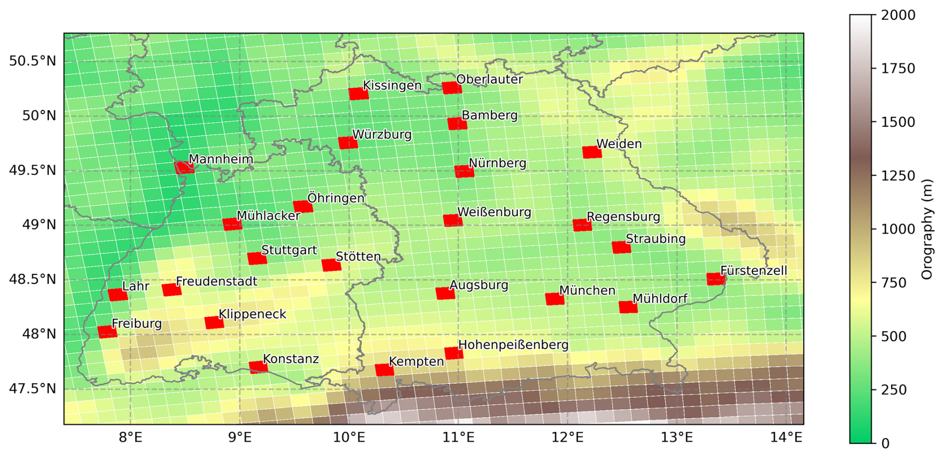
Figure 1 The study area of southern Germany with the topography of the CRCM5-LE grid, which has a resolution of 0.11°. The red gridcells indicate the selected grid cells of the climate simulations, which are extracted as the localities for our experiment.

2.2 The high-resolution large ensemble CRCM5-LE

To generate a single-model initial condition large ensemble, one single global climate model is run several times driven by a particular radiative forcing scenario. Small perturbations are applied to the initial conditions of each model run leading to different weather and climate realizations. The resulting ensemble spread can be interpreted as a model representation of internal climate variability (Deser et al., 2020). Large ensembles typically feature global climate models with spatial resolutions of several hundred kilometers, which is why they cannot represent extreme precipitation on sub-daily time scales. In our study, we employ the CRCM5-LE, a 50-member large ensemble dynamically downscaled over a European domain at a spatial resolution of 0.11° (approximately 12.5 km) from the global Canadian Earth System Model version 2 (CanESM2; Leduc et al., 2019). The dynamical downscaling is carried out over a European domain at a spatial resolution of 0.11° equaling 12.5 km.

The simulations of the CRCM5-LE extend from 1950 to 2099 and are driven by the high-emission scenario RCP8.5. We extract a 40-year time period from the recent past in 1980 to 2019, where Schwalm et al. (2020) report that total cumulative CO₂ emissions from 2005 to 2020 are in close agreement (within 1 %) with the RCP8.5 scenario. We simplifyingly assume stationarity for this 40-year period, which is in accordance with most operational extreme value models (Van de Vyver, 2012). We employ a Mann-Kendall test (Mann, 1945; Kendall, 1938) to evaluate the stationarity assumption in the 50 members of the CRCM5-LE. On a significance level of 95 %, only 6 % of the 50 CRCM5-LE members and all six durations show a significant trend, where 5 % show a positive trend. Hence, we follow that the assumption of stationarity is reasonable. Despite not explicitly simulating convection, the CRCM5-LE effectively captures the intensity of sub-daily rainfall extremes over Europe (Poschlod et al., 2021), showing good agreement with observations in the study area. In a brief evaluation, we test the CRCM5-LE data against observations from weather stations (Deutscher Wetterdienst, 2022) located within the periphery of CRCM5-LE grid points. The annual maxima of the CRCM5-LE data are extracted and the Generalized Extreme Value (GEV) distribution is fitted using L-moments, with 500 bootstrap samples of 28 years (matching the modal sample size of the observational data). We apply the Anderson-Darling test at α=0.05 on the GEV fits of the bootstrap parameters and the observations. For more on the Anderson-Darling test see Sect. 3.4.2 and the GEV see Sect. 3.1. Only 6 % of the fits are rejected indicating that the CRCM5-LE captures the characteristics of extreme precipitation across the durations well. Figure 2 displays the return levels of CRCM5-LE alongside observations from weather stations in Freudenstadt for all durations. The comparison demonstrates the good agreement between the two datasets (see Figs. S1–S25 in the Supplement for the other localities). This demonstrates that the model successfully captures the characteristics of extreme precipitation across various durations as well as its spatial variability between grid cells and observational stations.

It is very important to note, that we do not aim to extensively evaluate the performance of the CRCM5, for which there is ample literature (Poschlod et al., 2021; Poschlod, 2021). Instead, we use the CRCM5 as a “perfect model experiment” (Lenderink et al., 2023), assuming it as a perfect representation of the real climate system, where we know the “true” return level of the large ensemble. In this type of experiment, a climate model's large ensemble simulations, which sample a wide range of internal climate variability, are used as a proxy for a complete observational record. Thus, this experiment allows us to compare the performance of the different extreme value statistical models under idealized conditions. Hence, this experiment is referred to as “perfect model experiment” (Bevacqua et al., 2023).

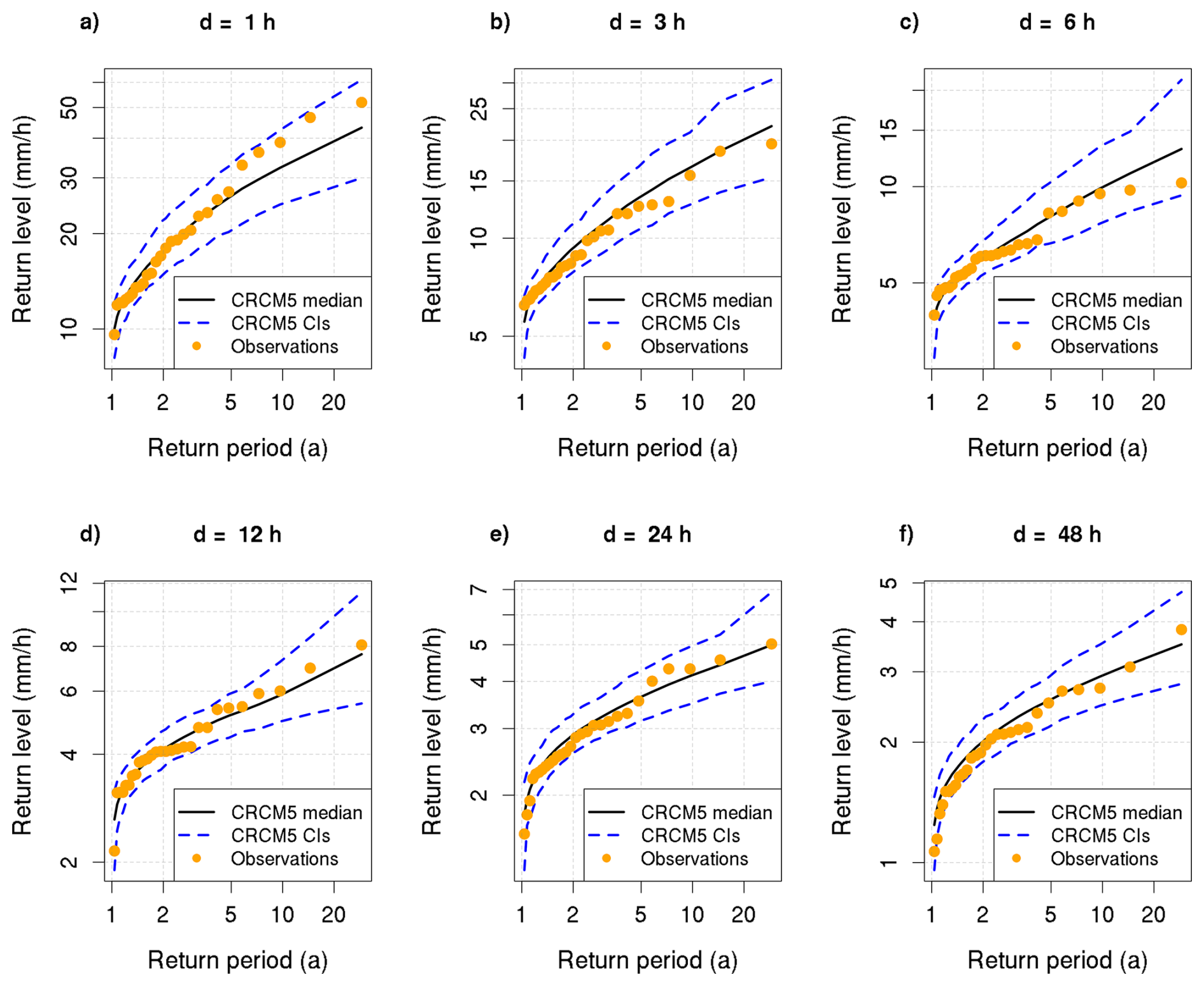
Figure 2 Return-level curves for the locality of Freudenstadt for durations (a) 1 h, (b) 3 h, (c) 6 h, (d) 12 h, (e) 24 h, (f) 48 h. Return level curves of CRCM5-LE are marked in the black line and 95 % confidence intervals in blue dashed line. The confidence intervals are obtained via bootstrap resampling. The annual maxima of the observational data (German weather service – Climate Portal) are plotted via Weibull plotting positions as the orange circles.

3 Methods

3.1 The Generalized Extreme Value distribution and its duration-dependent version

According to the Fisher-Tippett-Gnedenko theorem (Fisher and Tippett, 1928; Gnedenko, 1943), for sufficiently large blocks, the distribution of block maxima asymptotically follows the Generalized Extreme Value (GEV) distribution. The cumulative distribution function (CDF) of the GEV distribution is:

$$\begin{array}{}\text{(1)}& \begin{array}{rl}F(x;& {\mathit{\mu }}_{j,d},{\mathit{\sigma }}_{j,d},{\mathit{\xi }}_{j,d})=\\ & \exp \left\{-{\left[\mathrm{1}+{\mathit{\xi }}_{j,d}\left({\displaystyle \frac{x-{\mathit{\mu }}_{j,d}}{{\mathit{\sigma }}_{j,d}}}\right)\right]}_{+}^{-\mathrm{1}/{\mathit{\xi }}_{j,d}}\right\}\end{array}\end{array}$$

where μ_j,d is location parameter, σ_j,d is the strictly positive (${\mathit{\sigma }}_{j,d}>\mathrm{0}$) scale parameter and ξ_j,d is shape parameter for durations d and localities j. The shape parameter ξ governs the tail behavior and assigns the distribution to the reversed Weibull (${\mathit{\xi }}_{j,d}<\mathrm{0}$), Gumbel (${\mathit{\xi }}_{j,d}=\mathrm{0}$), or Fréchet (${\mathit{\xi }}_{j,d}>\mathrm{0}$) type. The duration-dependent GEV (dGEV) combines data from all durations into one model as it assumes that μ_j,d and σ_j,d follow a certain duration dependence (Koutsoyiannis et al., 1998; Fauer et al., 2021):

$$\begin{array}{}\text{(2)}& {\displaystyle }{\mathit{\sigma }}_j\left(d\right)={\mathit{\sigma }}_{\mathrm{0},j}(d+{\mathit{\theta }}_j{)}^{-{\mathit{\eta }}_j}\text{(3)}& {\displaystyle }{\mathit{\mu }}_j\left(d\right)={\stackrel{\mathrm{̃}}{\mathit{\mu }}}_j{\mathit{\sigma }}_{j,d}\end{array}$$

with ${\mathit{\sigma }}_j\left(d\right)>\mathrm{0},{\mathit{\sigma }}_{j,\mathrm{0}}>\mathrm{0},{\mathit{\theta }}_j>\mathrm{0},\mathrm{0}>{\mathit{\eta }}_j>\mathrm{0}$. Instead of modeling the durations separately, the duration dependency reduces to 4 parameters.

There are other versions of the dGEV, such as models that feature “multiscaling” (Gupta and Waymire, 1990). There, η is decomposed into two components η₁+η₂ rendering to $\mathit{\sigma }\left(d\right)={\mathit{\sigma }}_{\mathrm{0}}\cdot (d+\mathit{\theta }{)}^{-({\mathit{\eta }}_{\mathrm{1}}+{\mathit{\eta }}_{\mathrm{2}})}$. Fauer et al. (2021) found that the “multiscaling” dGEV is beneficial to cover a wide range of durations, i.e. 1 min to 5 d. However, in our study, we cover a range from 1 to 48 h, where the simple scaling approach is sufficient (see Fig. S51 in the Supplement).

3.2 Estimation methods

To cover the state-of-the-art procedures, we utilize four different estimation methods for fitting the statistical models. One of the estimation methods is L-moments estimation method, which are expectations of linear combinations of order statistics. They are analogous to conventional moments but can be estimated by linear combinations of order statistics, i.e. by L-statistics (Hosking, 1990). L-moments, being less sensitive to outliers, provide more robust and reliable estimates of the distribution's parameters, especially in small samples (Stedinger, 1993).

The Maximum Likelihood Estimation (MLE) method finds the values of the model parameters that maximize the likelihood function, which is a measure of how well the model explains the observed data. For a more comprehensive insight into the MLE see Coles et al. (2001), Martins and Stedinger (2000).

The Bayesian estimation method is a statistical method that uses prior knowledge with current data, which then updates in a posterior distribution of parameters (Zyphur and Oswald, 2015). From the posterior distribution we can obtain a measure of uncertainty. In Bayes' theorem, prior distribution is combined with the likelihood to produce the posterior distribution (see Eq. 4).

$$\begin{array}{}\text{(4)}& P\left(\mathit{\theta }\right|X)={\displaystyle \frac{P\left(X\right|\mathit{\theta }\left)P\right(\mathit{\theta })}{P\left(X\right)}}\end{array}$$

where P(θ|X) is the posterior distribution, P(X|θ) is the likelihood function, P(θ) is the distribution of the parameters called the “prior” and P(X) is the marginal likelihood, which normalizes the posterior distribution. We start with a prior distribution that reflects our initial knowledge about the parameter. Prior knowledge and observed data are synthesized when the prior is updated with the data through the likelihood function resulting in the desired posterior distribution. For a more in-depth analysis of Bayes' theorem we refer to Sivia and Skilling (2006) and Gelman et al. (2013). Choosing a prior is normally subjective and can be difficult without sufficient prior knowledge about the parameters (Berger, 1985). For estimation of the posterior parameters we use the No-U-turn sampler (NUTS), NUTS is an algorithmic enhancement of the Hamiltonian Monte Carlo (HMC) which uses the gradient information to sample from the target probability distribution (Hoffman and Gelman, 2014). In contrast, the commonly used the Metropolis-Hastings algorithm utilizes gradient-free random walk which is effectively “blind” to the distribution's geometry (Chib and Greenberg, 1995). For simplicity, we will refer to the samples generated by NUTS as “MCMC” samples.

When prior information is insufficient, Bayesian hierarchical models (BHMs) may be an alternative, as they can share a common hyperprior across a dimension (or many dimensions). In this way information is borrowed and learned from the data across the sites. The shared hyperprior centers a group of parameters, such as the means of normal distributions, around a common value (Gelman et al., 2013; Congdon, 2019). The central tendency of the hyperprior allows the model to shrink estimates toward a shared mean, therefore improving accuracy and robustness, particularly when data is sparse or noisy (Congdon, 2019). During inference, as data integrates into the model, individual group means tend to cluster around an empirically identified central value due to the hierarchical structure's information sharing across groups (Gelman, 2007; McElreath, 2015). Even when the hyperprior is uninformative or improper, shrinkage and balance toward a common mean can occur. In this process the BHM balances information from individual groups with the overall population. This mechanism enables the formulation of informed prior estimates for each site, using population-level data (Gelman et al., 2013; Congdon, 2019; Gelman, 2007). In the following example the Bayesian hierarchical model is set in three different tiers, which is typical for Bayesian hierarchical models (Gelman et al., 2013). A simple depiction of the BHM is as follows:

$$\begin{array}{ll}{\displaystyle }& {\displaystyle }\text{Data-Level:}{y}_j\mid {\mathit{\theta }}_j,\mathit{\varphi }\sim P(y_j\mid {\mathit{\theta }}_j,\mathit{\varphi })\\ {\displaystyle }& {\displaystyle }\text{Parameter Level:}{\mathit{\theta }}_j\mid \mathit{\varphi }\sim P({\mathit{\theta }}_j\mid \mathit{\varphi })\\ {\displaystyle }& {\displaystyle }\text{Hyperparameter Level:}\mathit{\varphi }\sim P\left(\mathit{\varphi }\right)\end{array}$$

where $P(y_j\mid {\mathit{\theta }}_j,\mathit{\varphi })$ is the likelihood, P(θ_j∣ϕ) is the prior distribution and P(ϕ) is the hyperprior distribution. See Congdon (2019) for a more comprehensive overview of Bayesian hierarchical models.

3.3 The applied EVT models

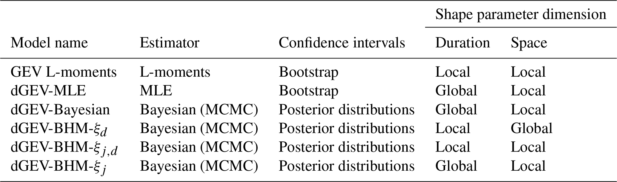
We apply six different models in order to evaluate their performance. Two frequentist and four Bayesian models make up our repertoire. As a summary, we provide an overview of the six different EVT models in Table 1.

3.3.1 The frequentist models

In our first frequentist model we use a standard GEV, where the equation is expressed in Eq. (1). As this model is not duration-dependent, we model each duration separately. Additionally, since this model is not hierarchical, we also model the locations separately. This results in six GEV models for each duration and for 25 separate locations, totaling 150 GEV models. We use the R package extRemes (Gilleland and Katz, 2016) to apply the L-moments estimation method for this as described in Sect. 3.2. As a second frequentist model we apply the dGEV, which incorporates duration dependence as outlined in Eqs. (2) and (3). This combines all the durations into one dGEV model for each locality equaling 25 dGEV models in total. As implemented in the R package IDF (Fauer et al., 2022), we use the MLE to estimate this model and refer to it as dGEV-MLE. We generate confidence intervals for both frequentist models using a nonparametric bootstrap with a sample size of 500 (Efron and Tibshirani, 1994), resampling the annual maxima with replacement.

3.3.2 The duration-dependent Bayesian GEV

In the Bayesian duration-dependent generalized extreme value distribution (dGEV-Bayesian) model, we employ distinct priors for the parameters of each location. These priors do not share a hyperprior, thus the model is not hierarchical. Each parameter has a prior normal distribution, with the mean of these priors based on estimates for the corresponding dGEV-MLE parameters.

$$\begin{array}{}\text{(5)}& {\displaystyle }\stackrel{\mathrm{̃}}{\mathit{\mu }}& {\displaystyle }\sim N({\stackrel{\mathrm{̃}}{\mathit{\mu }}}_{\left(\mathrm{MLE}\right)},\mathrm{10})\text{(6)}& {\displaystyle }{\mathit{\sigma }}_{\mathrm{0}}& {\displaystyle }\sim N({\mathit{\sigma }}_{\mathrm{0},\left(MLE\right)},\mathrm{10})& {\displaystyle }T[\mathrm{0},]\text{(7)}& {\displaystyle }\mathit{\xi }& {\displaystyle }\sim N({\mathit{\xi }}_{\left(\mathrm{MLE}\right)},\mathrm{5})& {\displaystyle }T[-\mathrm{0.5},\mathrm{0.5}]\text{(8)}& {\displaystyle }\mathit{\theta }& {\displaystyle }\sim N({\mathit{\theta }}_{\left(\mathrm{MLE}\right)},\mathrm{10})& {\displaystyle }T[\mathrm{0},]\text{(9)}& {\displaystyle }\mathit{\eta }& {\displaystyle }\sim N({\mathit{\eta }}_{\left(\mathrm{MLE}\right)},\mathrm{5})& {\displaystyle }T[\mathrm{0},\mathrm{1}]\end{array}$$

As σ₀, θ and η are limited parameters, we devise truncated normal distributions. These are normal distributions where either the upper end or lower end is truncated, denoted as T[lower end,upper end]. We limit normal distribution for ξ between −0.5 and 0.5, which is common practice and recommended for the shape parameter (Martins and Stedinger, 2001; Papalexiou and Koutsoyiannis, 2013). Given that ξ and η are restricted to a narrow range, we devise smaller variances in the normal priors. We derive confidence intervals from the posterior parameter distributions with 500 MCMC iterations.

3.3.3 Bayesian hierarchical duration-dependent generalized extreme value distribution

Here we introduce the Bayesian hierarchical duration-dependent GEV (in short: dGEV-BHM). In the dGEV-BHM, all stations and durations are incorporated into a single comprehensive model. This model is different from the previously mentioned models, as its parameters share hyperparameters over space and/or durations, making it hierarchical. The base of our model is that of the dGEV (see Eqs. 2 and 3) with different variations in the dimensions of the shape parameter ξ. We have three different versions of this model: dGEV-BHM-ξ_d, dGEV-BHM-ξ_j and dGEV-BHM-ξ_j,d.

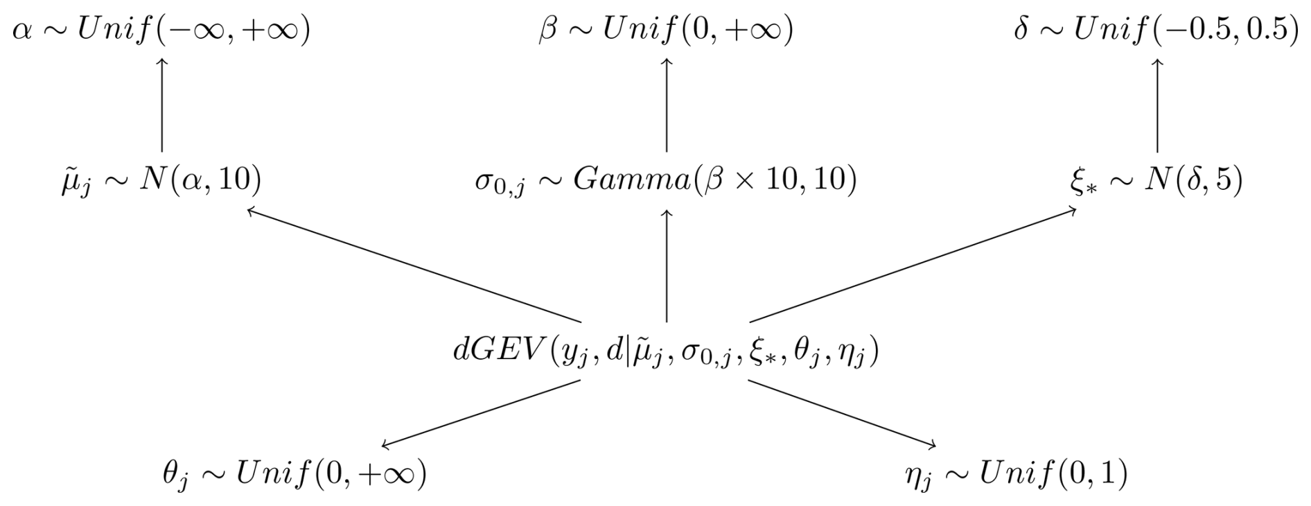
Figure 3 Diagram of the dGEV-BHM. We devise three different variations of the dGEV-BHM, where the shape parameter ${\mathit{\xi }}_{*}\in \mathit{\{}{\mathit{\xi }}_d,{\mathit{\xi }}_{j,d},{\mathit{\xi }}_j\mathit{\}}$.

In all models, the rescaled location parameter and scale offset share a hyperparameter over space α and β. $\stackrel{\mathrm{̃}}{\mathit{\mu }}$ has normal prior, with a standard deviation of 10 and the mean is the hyperprior α.

$${\stackrel{\mathrm{̃}}{\mathit{\mu }}}_j\sim N(\mathit{\alpha },\mathrm{10})$$

where α is an uninformative hyperprior. For the scale offset σ_0,j we use a Gamma distribution, with its shape parameter equal β⋅10 and the inverse scale (or “rate”) parameter equal to 10. In that way, we ensure that the mean of the distribution is equal to β.

$${\mathit{\sigma }}_{\mathrm{0},j}\sim \text{Gamma}(\mathit{\beta }\cdot \mathrm{10},\mathrm{10})$$

For the spread of the priors we performed a prior selection process to find a well-performing and stable model. We found that narrow spreads led to convergence issues, as this constrained the model too much. On the other hand, wide spreads yielded performance that was similar to to the chosen parameters. A standard deviation of 10 was selected for the Normal distribution, as this value proved stable in preliminary tests. The Gamma prior was parameterized as Gamma(Kβ,K) to ensure its mean remained fixed at the hyperprior value β. The concentration parameter K was set to 10, as this value was stable in our tests. We chose a preliminary prior selection process rather than a full prior sensitivity analysis due to the large computational demand with many sub-samples.

Uninformative (improper) hyperpriors allow the data to drive inferences, especially when there is little prior information available (Banerjee and Fuentes, 2012; Cooley et al., 2007). It can still facilitate information sharing across groups through partial pooling and shrinkage effects (Röver and Friede, 2020). Partial pooling allows information to be partially shared between groups, resulting in parameter estimates that are a weighted average of the group-level data and the overall population estimate. Shrinkage effects pull the estimates of group-level parameters towards the overall population mean. This combination allows for data-driven inference while still benefiting from the hierarchical structure of the model, which is particularly useful when prior knowledge is limited.

The innovative aspect of this distribution is that we model the shape parameter of the dGEV distribution, used to model the block maxima of rainfall durations, in three distinct ways:

1. Hierarchical over duration (ξ_d): The shape parameter varies systematically with the duration under consideration.

2. Hierarchical over space (ξ_j): The shape parameter changes based on the geographical locality.

3. Hierarchical over both space and duration (ξ_j,d): The shape parameter depends on both the duration and the locality.

For all these variations of the shape parameter, we assume a normal distribution with a narrower standard deviation of 5 and a hyperparameter denoted as δ.

$${\mathit{\xi }}_{\ast }\sim N(\mathit{\delta },\mathrm{5})$$

The hyperparameter δ itself follows a weakly informative uniform distribution constrained between −0.5 and 0.5:

$$\mathit{\delta }\sim \text{Uniform}(-\mathrm{0.5},\mathrm{0.5})$$

This setup facilitates partial pooling of information, either through duration, location, or both. Partial pooling allows information to be shared between groups or durations, resulting in more robust estimates of the shape parameter, particularly in cases with limited data. The weakly informative prior on δ ensures that the model remains data-driven while still benefiting from the hierarchical framework. We derive confidence intervals from the posterior parameter distributions of the three versions of the dGEV-BHM, with 500 MCMC iterations each.

Table 1 Table of all six EVT models and their estimation method, generation of the confidence intervals and shape parameter dimension (space and/or duration). Shape parameter dimensions: Global = one shape parameter spanning across the dimension indices. Local = several shape parameters across dimension indices.

3.4 Goodness of fit and evaluation

3.4.1 Sub-sampling strategy

Our aim is to use the large sample size of the CRCM5-LE to evaluate the ability of the six different EVT models to reproduce rare rainfall return levels. Therefore, we randomly sample smaller sub-samples of $\mathit{\{}\mathrm{30},\mathrm{40},\mathrm{\dots },\mathrm{90},\mathrm{100}\mathit{\}}$ years from the 2000-year CRCM5-LE population. Each sub-sample is randomly drawn 100 times. We then fit the six EVT models to the sub-samples and compare the resulting EVT model outputs to the effective return level of the full 2000-year CRCM5-LE.

3.4.2 Anderson Darling

The Anderson Darling (AD) test is a method which analyzes how well empirical data fits a theoretical distribution. It is a modification of the Kolmogorov-Smirnov (K-S) test and is more sensitive to discrepancies in the tails (Stephens, 1974), making it suitable to assess extreme value distributions. The mathematical formulation for the AD test is:

$$\begin{array}{}\text{(10)}& {\displaystyle }{A}^{\mathrm{2}}=-n-S\text{(11)}& {\displaystyle }\begin{array}{rl}S& =\sum _i\left[(\mathrm{2}i-\mathrm{1})/n\right]\\ & \cdot \left[\ln F\left(X_i\right)+\ln (\mathrm{1}-F(X_{n-i+\mathrm{1}}\left)\right)\right]\end{array}\end{array}$$

where n is the sample size, i is the sample index (ordered lowest to highest) and F(X) is the cumulative distribution. Thus, S is the discrepancy between the empirical cumulative distribution and the theoretical cumulative distribution, whereby more weight is applied to the differences at the tails of the distribution. The p-value quantifies the evidence against the hypothesis that the data follows the specified distribution and is commonly obtained from tabulated critical values. However, in this study, we compute the p-value from the Anderson-Darling test statistic itself using piecewise exponential approximations as implemented in the R package gnFit (Saeb, 2018).

We apply the AD test at the significance α=0.05. The Anderson-Darling (AD) test is a method commonly applied to evaluate the goodness of fit for the GEV distribution, especially when fitted to annual maxima of precipitation. However, the AD test can only evaluate the quality of the fit between the theoretical GEV distribution and the empirical distribution of the block maxima samples. Although the test's p-value may indicate a good fit for a given dataset, it does not guarantee that the model will produce accurate extreme, unseen quantiles. The test also cannot assess how well a limited empirical sample represents the full population of possible extreme rainfall events governed by internal climate variability (Poschlod, 2021). The true performance of an extreme value model lies in its ability to accurately estimate rare return levels that are critical for risk assessment.

For this reason, while distributional tests like the AD test are useful for initially checking the fit, we also evaluate if they are sufficient as the sole metric for validating extreme value models, particularly when the goal is to evaluate tail risk. Our aim is therefore not to validate the models with the AD test, but to investigate if it is reliable in estimating extreme quantiles, which we will assess using our tail risk metrics, introduced in Sect. 3.4.5. To do this, we apply the AD test on the 100 sub-samples of 30 to 100 years generated from the CRCM5-LE population (mentioned in Sect. 3.4.1) and assess the respective GEV and dGEV parameter estimates of each duration and location. In total 720 000 hypothesis tests ($\mathrm{8}\text{ sub-sample ranges}\times \mathrm{100}\text{ sub-samples}\times \mathrm{25}\text{ localities}\times \mathrm{6}\text{ durations}$) are performed, and from this, the proportion of tests fulfilling p>0.05 is determined.

3.4.3 Akaike information criterion

The Akaike information criterion (AIC) is a statistical measure for model selection that balances goodness-of-fit with its complexity (Sakamoto et al., 1988). It aims to achieve “parsimony” in a model by selecting the model that balances complexity and likelihood. To effectively use the AIC, it must be applied to a set of candidate models that have been fitted to the same data. The model with the lowest AIC is then chosen as the preferred model (Anderson et al., 1998). The formula for the AIC is:

$$\begin{array}{}\text{(12)}& \mathrm{AIC}=\mathrm{2}k-\mathrm{2}\log \left(\widehat{L}\right)\end{array}$$

where k represents the number of estimated parameters, serving as a measure of the model's complexity. This term acts a penalty to help prevent overfitting, which is a common issue where a model fits the training data too closely but fails to generalize to new data. $\widehat{L}$ is the maximum value of the likelihood function for the model, which quantifies how well the model fits the data. Hence, the AIC thereby relies on a single maximum likelihood estimate, whereas the four Bayesian models in our study provide a full posterior distribution of parameters via MCMC instead of a single point estimate. Therefore, as a workaround, we use the posterior means of the Bayesian models for the AIC calculation. In turn, the widely applicable information criterion (WAIC) utilizes the entire posterior distribution of Bayesian models. However, it is only applicable to Bayesian models. As our model setup features four Bayesian models and two frequentist models, we provide the AIC as a consistant measure across all six models and include the WAIC in the supplement.

3.4.4 Effective return levels

An important foundation of this study is the use of effective return levels, which we directly infer from the 2000-year large ensemble. We derive effective return levels, such as the 100-year return level represented by the 20th highest index (n₍₂₀₎) and the 10-year return level represented by the 200th highest index (n₍₂₀₀₎). To obtain a robust estimate of the effective return level with a measure of uncertainty, we employ a bootstrapping procedure, resampling the entire dataset 500 times with replacement. By computing the return levels from the sub-samples via the six EVT models (see Table 1) and comparing them to the effective return levels from the full CRCM5-LE sample, we can determine how accurately each statistical model replicates the ensemble data. This procedure is paramount for validating the models' reliability and robustness.

3.4.5 Error metrics: relative error and return level concordance

We assess the accuracy of an EVT model, by calculating the relative error (RE) between the modeled return level and the effective return level. Therefore, for a given return period, we determine the percentage difference between the model return level and the effective return level. For each EVT model, we compute the RE for 10- and 100-year return levels for sub-samples sizes ranging between 30 and 100 years. Furthermore, we assess the 80 % confidence intervals derived via bootstrapping for the frequentist models and the posterior parameter distribution for the Bayesian models on each of the 100 sub-samples. Thereby, we assess the uncertainty ranges indicating the robustness of the EVT models. The choice of 80 % confidence intervals helps visualize the RE better in the figures.

The return level concordance (RLC) describes the agreement between the EVT model's computed return levels from the 100 sub-samples and the confidence intervals derived from the large ensemble climate data. The RLC quantifies the fraction of the EVT model 100-year return levels that are within the 95 % confidence interval of the effective 100-year return level (see Fig. 4).

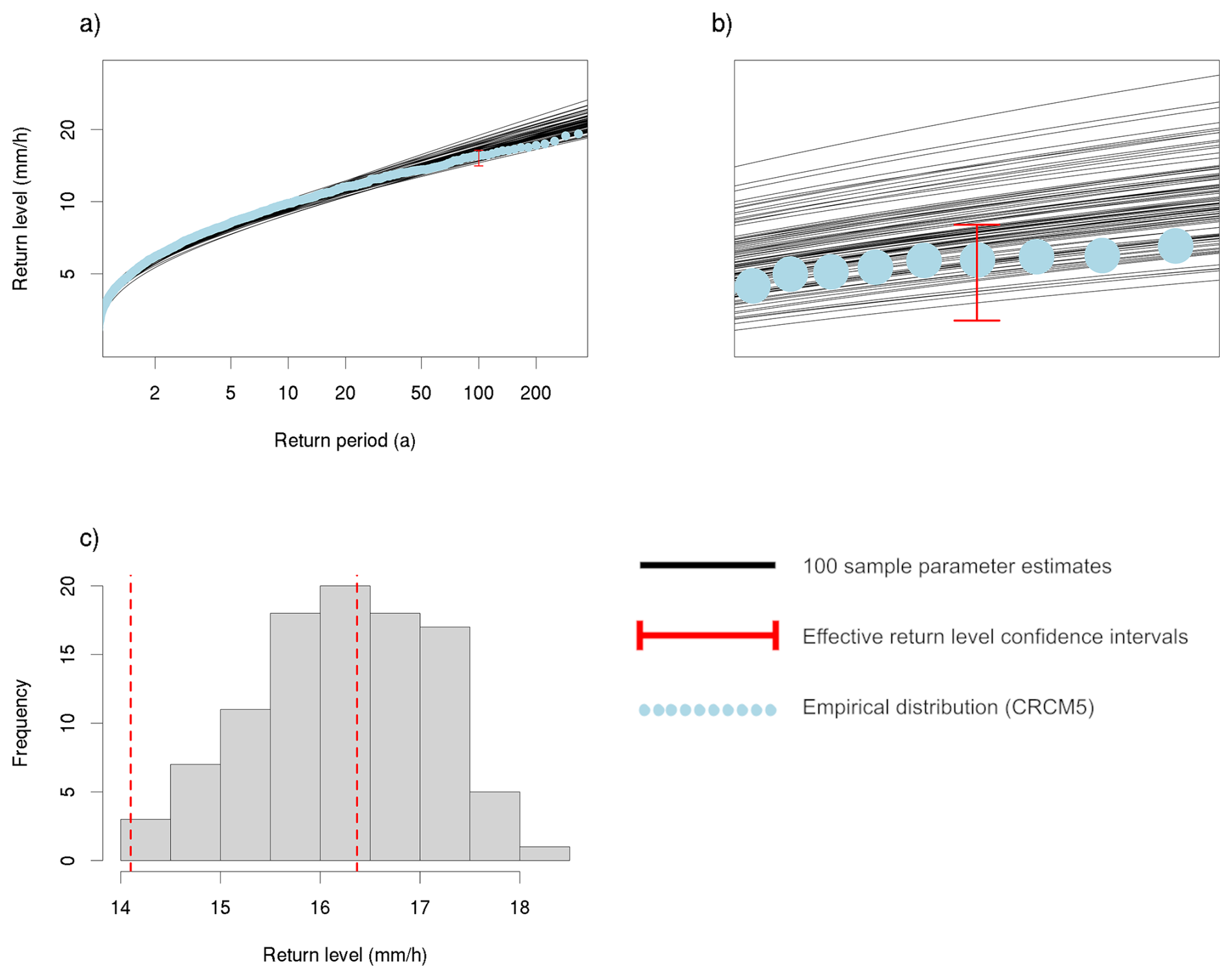
Figure 4 Conceptual representation of the 100-year return level concordance (RLC) for one locality (Augsburg) and duration (6 h) and sub-sample of 40 years. (a) The return levels based on a EVT model (black lines) are compared to the confidence interval (red bar) of the effective 100-year return level, which is derived from the full 2000-year CRCM5-LE (light blue dots). (b) Zoom-in to the RLC at the 100-year return level. In this example the RLC would amount to 55 %. (c) Histogram of the RLC, the red dashed lines are the confidence intervals of the effective 100-year return level.

3.5 Intensity-duration-frequency (IDF) curves

Lastly, we construct IDF curves from the parameter estimates of dGEV models. The rainfall return level at a given duration d and return period T is:

$$\begin{array}{}\text{(13)}& {\displaystyle }x\left(T\right)=\mathit{\mu }\left(d\right)+{\displaystyle \frac{\mathit{\sigma }\left(d\right)}{\mathit{\xi }}}\times \left\{{\left[-\log (\mathrm{1}-\mathrm{1}/T)\right]}^{-\mathit{\xi }}-\mathrm{1}\right\}\end{array}$$

where ξ is the shape parameter, and σ(d) and μ(d) are the scale and location parameters respectively given at specific durations. The scale offset σ₀ and rescaled location parameter $\stackrel{\mathrm{̃}}{\mathit{\mu }}$ are both incorporated into the duration-dependent parameters (Koutsoyiannis et al., 1998; Fauer et al., 2021):

$$\begin{array}{}\text{(14)}& {\displaystyle }\mathit{\sigma }\left(d\right)& {\displaystyle }={\mathit{\sigma }}_{\mathrm{0}}\times (d+\mathit{\theta }{)}^{-\mathit{\eta }}\text{(15)}& {\displaystyle }\mathit{\mu }\left(d\right)& {\displaystyle }=\stackrel{\mathrm{̃}}{\mathit{\mu }}\times \mathit{\sigma }\left(d\right)\end{array}$$

In the Bayesian hierarchical models both the scale offset σ₀ and rescaled location parameter $\stackrel{\mathrm{̃}}{\mathit{\mu }}$ share hyperparameters across space. In the two models dGEV-BHM-ξ_d and dGEV-BHM-ξ_j,d the shape parameter ξ_d is modeled along the duration d, and therefore requires interpolation to construct the resultant IDF curve between the discrete durations. To construct a continuous IDF curve between the durations, an initial approximation is generated by linearly interpolating the mean of the shape parameter ξ between the discrete durations. This preliminary curve is then modified using an adjustment step. The required adjustment – defined as the difference between the approximate curve and the actual quantiles calculated using the full posterior distribution of ξ at the discrete durations – is then interpolated and applied to the initial curve.

4 Results

4.1 Anderson-Darling test

First, we present the results of the AD test, as the goodness-of-fit evaluation would be the typical next step after the fitting of EVT models. Figure 5 illustrates the fraction of passed AD tests for all 25 localities, 6 durations, and 100 sub-samples across the 8 sub-sample sizes between 30 and 100 years. Given the significance level of α=0.05, a 95 % fraction of passed AD tests would be expected if all data samples came from the tested theoretical distribution specified by the EVT model fits. We see that the overall test results decrease with increasing sample sizes, as the AD test gains more power to reject the null hypothesis detecting deviations between the sample and the theoretical distribution (Shin et al., 2012). The AD test diagnoses the highest rejection rates for the dGEV-BHM-ξ_d. The dGEV-BHM-ξ_j, dGEV-Bayesian, and dGEV-MLE reach 95 % acceptance for 30-year samples dropping to 93 % for 100-year samples. The dGEV-BHM-ξ_j,d and GEV-Lmoments show the lowest rejection rates. We note that this performance can be linked to the flexibility of the EVT models. The GEV-Lmoments estimates location, scale, and shape parameters separately for each locality and duration providing the highest flexibility to fit the GEV to the samples. With the duration dependence, the dGEV limits the flexibility. The dGEV-BHM-ξ_j,d is the most flexible version allowing the shape parameter to vary over space and duration (see Table 1). In turn, the dGEV-BHM-ξ_d fixes the shape parameter over space resulting in the highest rejection rate of the AD test.

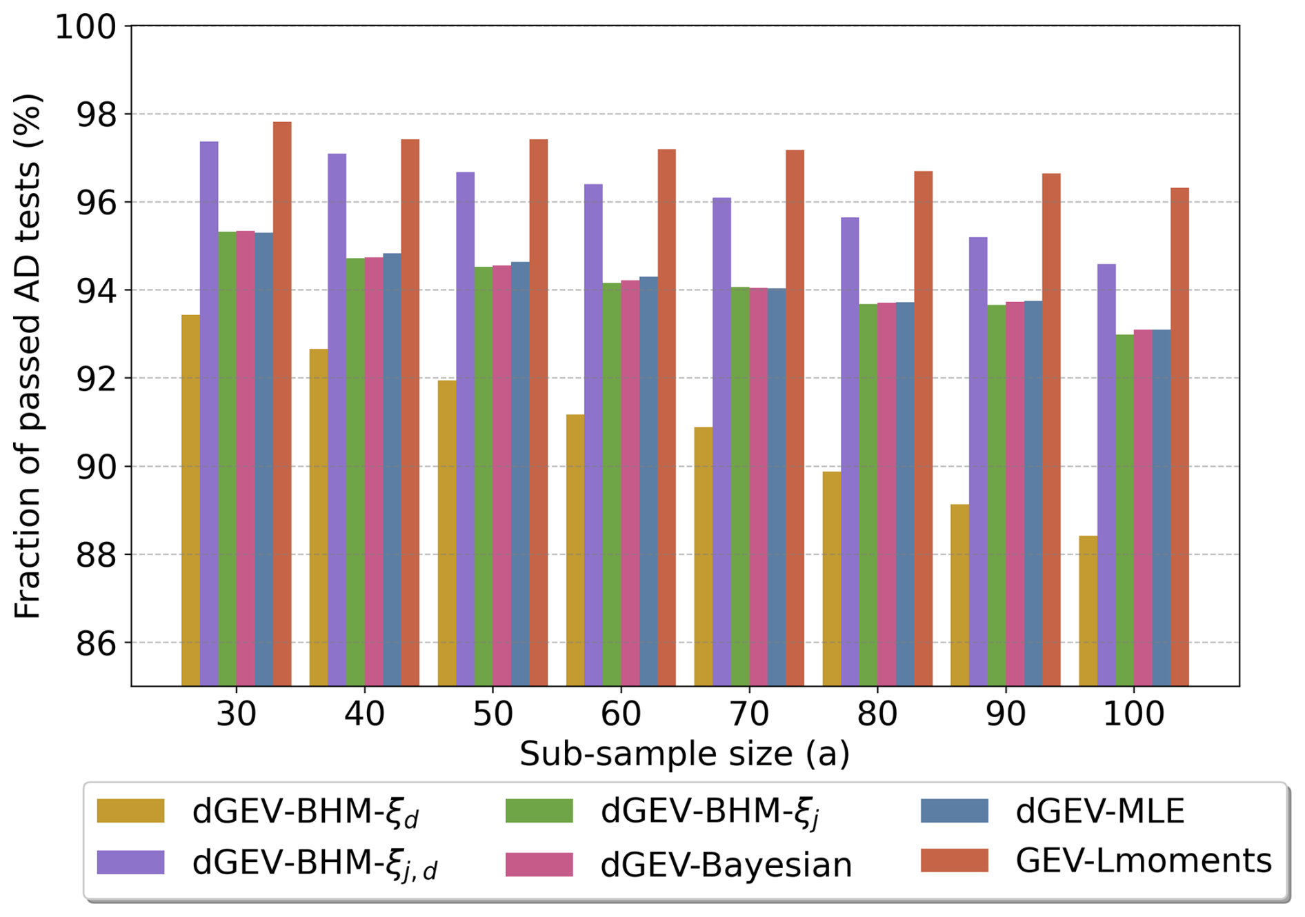
Figure 5 Fraction of passed Anderson-Darling tests for the six EVT models and 100 sub-samples at sizes reaching from 30 to 100 years. The fractions are averaged over the 25 localities and 6 durations.

4.2 Akaike information criterion

The average ranks according to the AIC values are illustrated in Fig. 6. The dGEV-BHM-ξ_d model consistently ranks first (the lowest average rank) across all sub-sample sizes, indicating it is the best model choice according to the Akaike Information Criterion (AIC).

The second best model is dGEV-BHM-ξ_j, which has the second-lowest average rank across all sub-sample sizes. Following that, dGEV-Bayesian and dGEV-MLE are the third and fourth best, respectively. The dGEV-BHM-ξ_j,d and GEV-Lmoments models consistently rank as fifth and sixth, respectively.

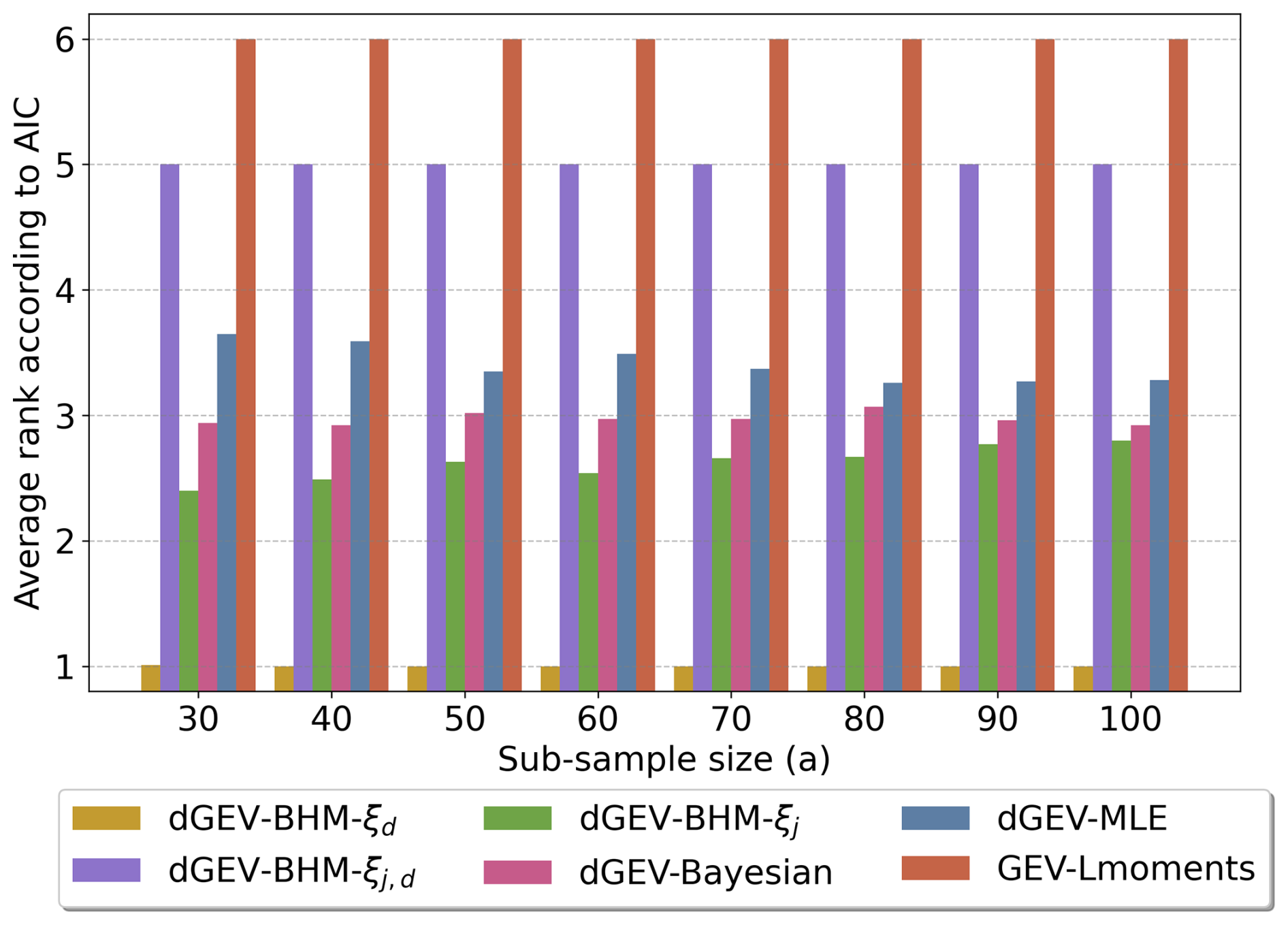
Figure 6 Average ranks according to the AIC values for all models and all their sub-sample sizes.

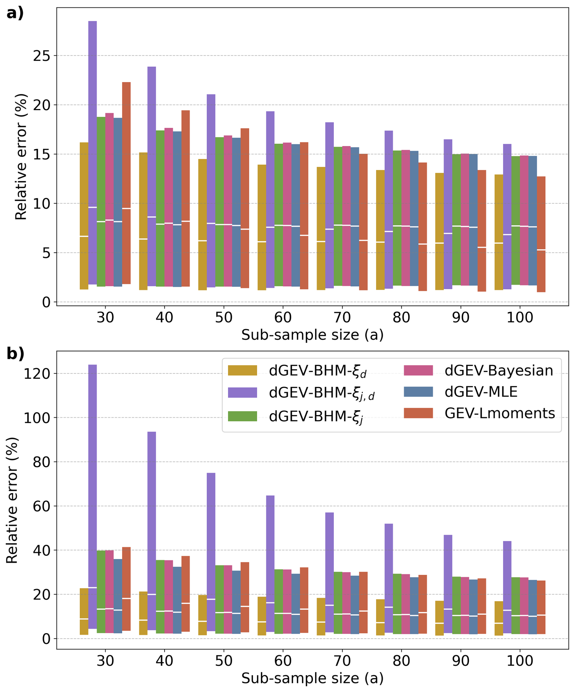
Figure 7 The relative error (RE) of the (a) 10-year return levels and (b) 100-year return levels averaged across all localities and durations. The bars indicate the range of the inner 80 % of the 100 sub-samples and 500 bootstrap or MCMC iterations, where the white marker represents the median.

4.3 Relative error

The relative error is presented in Fig. 7 for 10-year and 100-year return levels. The performance of EVT models reveals distinct patterns across varying sub-sample sizes. For the 10-year RE (Fig. 7a)], dGEV-BHM-ξ_d consistently demonstrates superior performance across sub-sample sizes up to 70 years, with GEV-Lmoments showing the lowest RE for sample sizes of 80 to 100 years. The dGEV-BHM-ξ_j, dGEV-Bayesian, and dGEV-MLE score very similarly and show low sensitivity to the sample size. Conversely, the dGEV-BHM-ξ_j,d model exhibits the poorest performance for low sample sizes up to 50 years, but improves for larger samples. In contrast, for the 100-year RE (Fig. 7b), dGEV-BHM-ξ_d consistently emerges as the most accurate model across all sub-sample sizes. The dGEV-BHM-ξ_j,d and GEV-Lmoments are identified as the least accurate. Again, dGEV-BHM-ξ_j, dGEV-Bayesian, and dGEV-MLE show an equivalent accuracy. The robustness of the six EVT models behaves similar for the 10-year and 100-year return levels. The error ranges of the dGEV-BHM-ξ_j,d are by far the largest showing high sensitivity to the sample size. In turn, the dGEV-BHM-ξ_d is diagnosed the most robust model consistently across the sub-sample sizes.

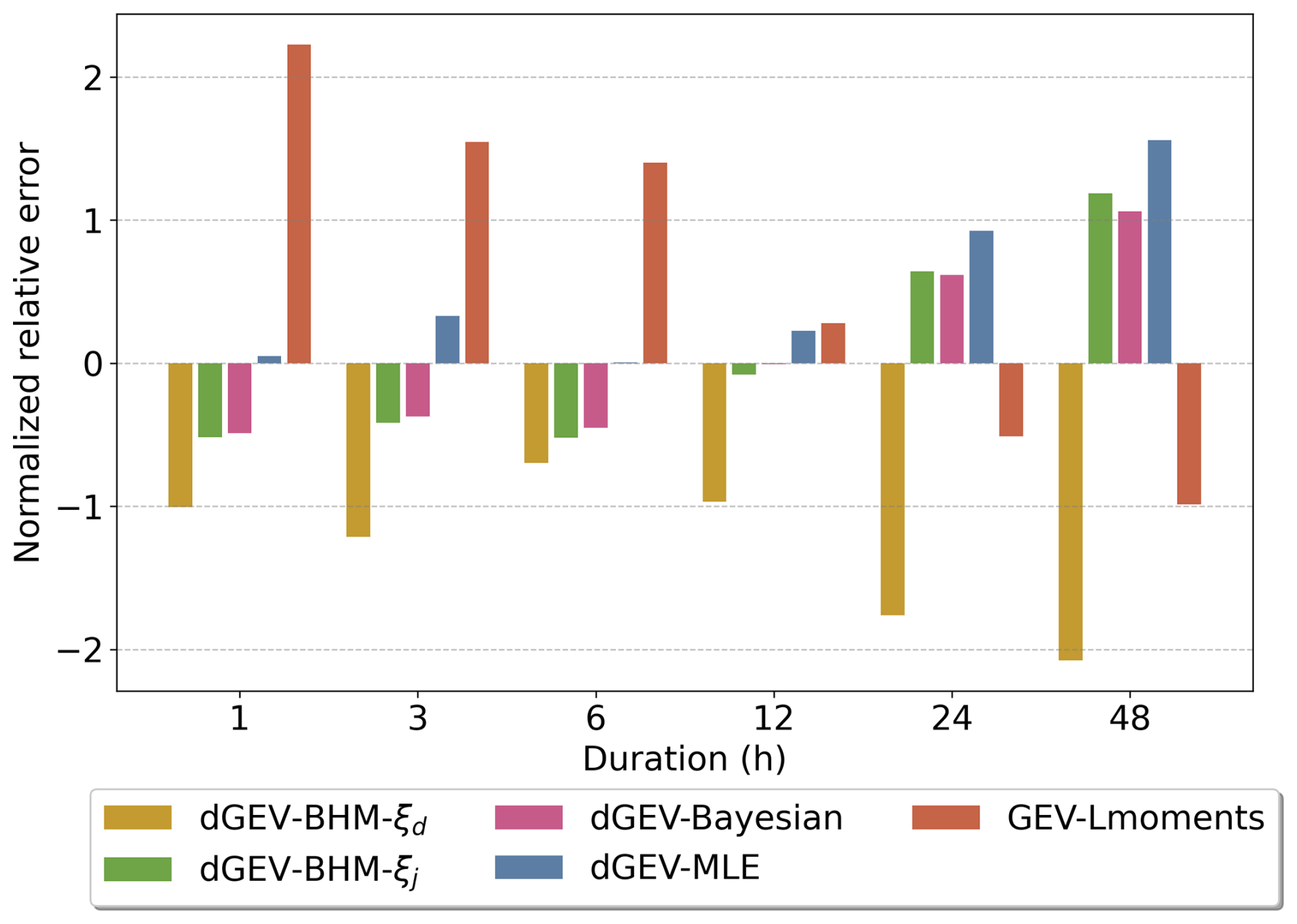
Figure 8 Average 100-year relative error (RE) across durations for sub-sample size of 30 years. Note that the the dGEV-BHM-ξ_j,d is not shown as the high REs distort the standardized results.

In Fig. 8 we present the location average 100-year RE for sub-sample size n=30 at different durations. We normalize the RE for each model across five models for each duration. We intentionally leave the dGEV-BHM-ξ_j,d out, as the results of RE are so high that they distort the standardized results. Across all durations, the dGEV-BHM-ξ_d consistently shows the lowest RE. GEV-Lmoments shows high errors for the short durations of 6 h and below, but comparably low REs for 24 and 48 h. In contrast, dGEV-BHM-ξ_j, dGEV-Bayesian, and dGEV-MLE show the tendency to perform better for shorter than for longer durations.

4.4 Return level concordance

Figure 9 features the RLC for the 100-year return level. For all six EVT models, the RLC increases with increasing sample size. The dGEV-BHM-ξ_d can achieve the highest RLC between 27 % and 35 % outperforming the other five EVT models by around 10 %, proving its robustness. The dGEV-BHM-ξ_j, dGEV-Bayesian, and dGEV-MLE perform similarly in a range from 17 % to 24 %. In contrast, both the dGEV-BHM-ξ_j,d and GEV-Lmoments consistently exhibit the lowest RLC between 10 % and 22 %.

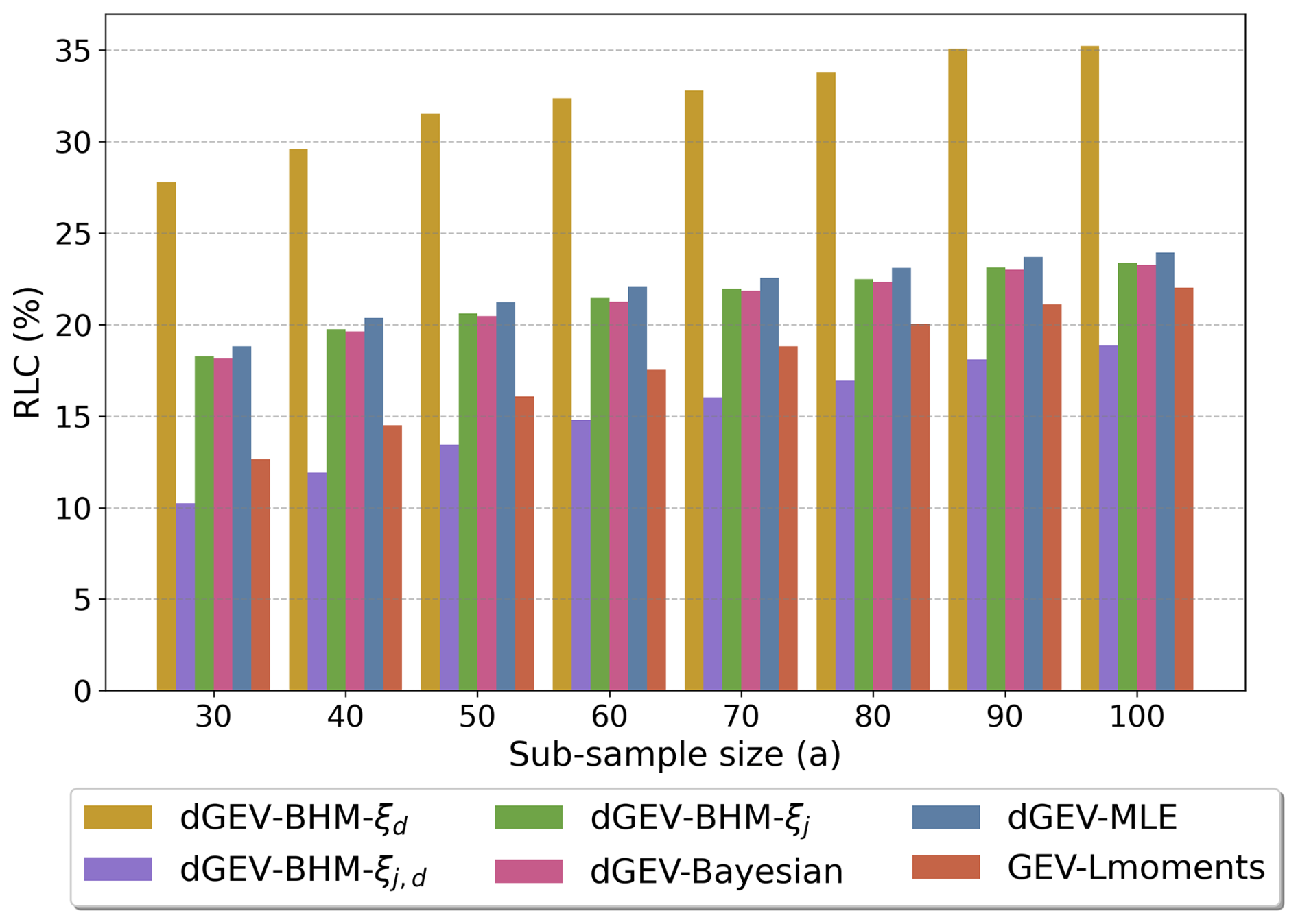
Figure 9 Return level concordance (RLC) for 100-year return levels, for the six EVT models and sub-sample sizes ranging from 30 to 100 years. The RLC is averaged over the localities and durations.

4.5 Intensity-duration-frequency (IDF) curves

Figure 10 illustrates IDF curves for the best performing model dGEV-BHM-ξ_d and the state-of-the-art dGEV-MLE for one example locality in Würzburg (see Figs. S26–S50 in the Supplement for the IDF curves of the other localities). The IDF curves are constructed on the sub-sample size of n=30 reflecting typical data availability for sub-daily rainfall durations in Germany. In this case, the dGEV-BHM-ξ_d can reproduce the 100-year return levels across all durations, while the dGEV-MLE overestimates for the durations of 6 h and above. The 95 % confidence intervals of the dGEV-BHM-ξ_d are narrower than for the dGEV-MLE indicating its robustness even under data scarce conditions.

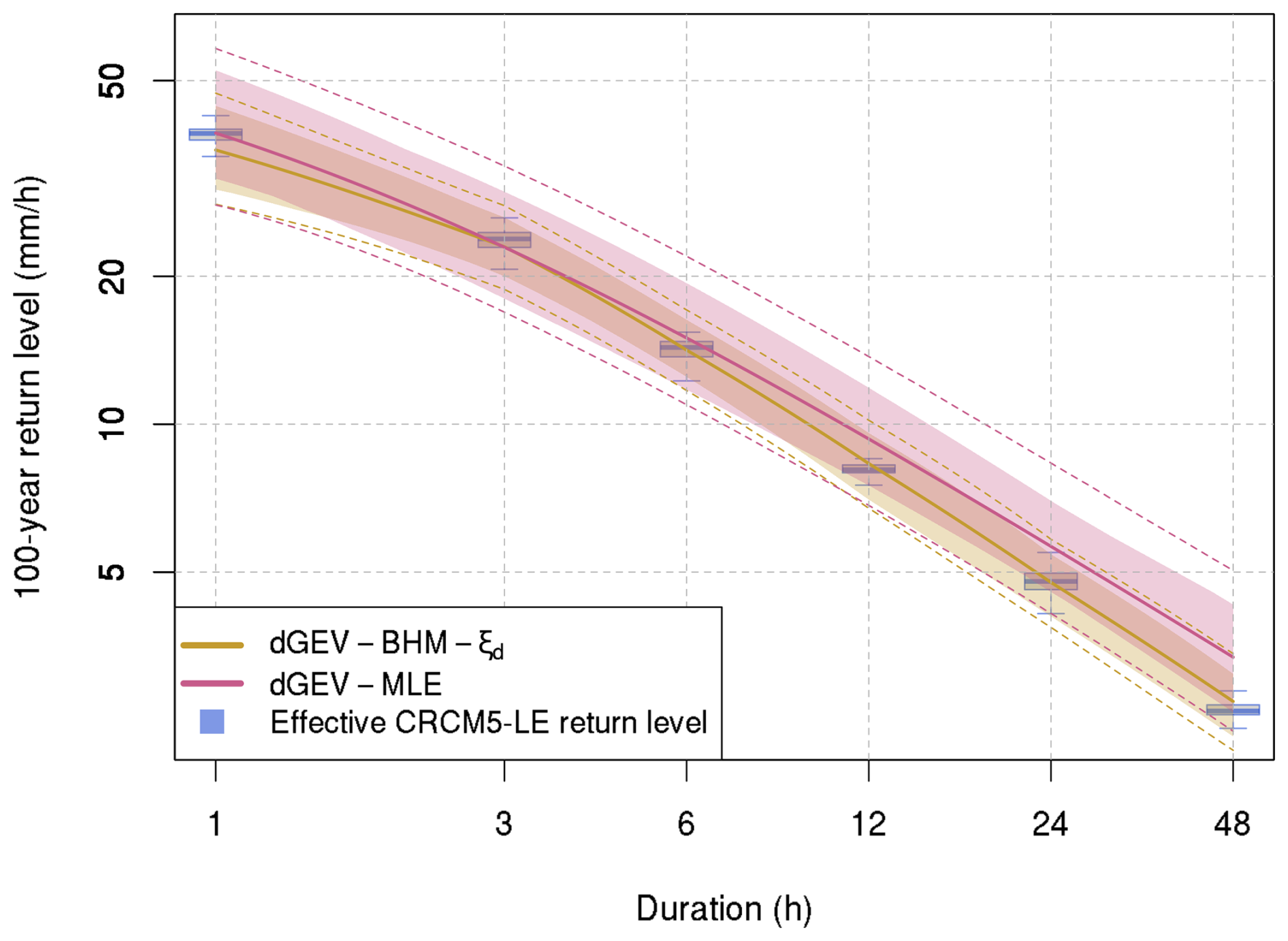
Figure 10 IDF curves of the dGEV-BHM-ξ_d and dGEV-MLE for the locality Würzburg and the 100-year return period. IDF curves are constructed based on a sub-sample size of 30 years. The dashed lines depict the 95 % confidence intervals for all 100 sub-samples and combined MCMC/Bootstrap iterations, whilst the polygons represent the 95 % confidence intervals for the 100 sub-sample means. The boxplots represent the ranges of the 100-year return level derived from resampling the 2000-year CRCM5-LE with replacement.

5 Discussion

5.1 Goodness-of-fit and information criteria

Our experiment reveals that the rejection rates of the Anderson-Darling test align with the flexibility of the EVT models, where more flexible models are rewarded by lower rejection rates. Conversely, the dGEV-BHM-ξ_d showing the highest rejection rates performs better than the other models in terms of the RE and RLC. Hence, we argue that the AD test on small samples of 30 to 100 years is not well-suited to assess the quality of how well an EVT model fits the full sample of 2000 years. We attribute this observed pattern to a lack of robustness to internal climate variability. Specifically, if a small sample, due to random sampling, does not accurately represent the full 2000-year sample, flexible EVT models are prone to overfitting it. This is rewarded by a successful AD test on the small sample, but diagnosed by a potential higher RE and lower RLC when considering the full 2000-year sample. This is a clear manifestation of the bias-variance trade-off: more flexible models have lower bias but higher variance, leading to poor generalization. While a practitioner with a limited observational sample may only see a good AD test result and interpret it as model success, our study demonstrates the inherent limitation of this goodness-of-fit testing when evaluating the true performance of extreme quantiles. Hence, this is driven by the variability of the annual maxima of precipitation within the 2000-year sample. The source of this variability is the chaotic nature of the climate system, or in other words, internal climate variability, which is a huge source of uncertainty in assessments of extreme precipitation (Aalbers et al., 2018; Bhatia and Ganguly, 2019; Martel et al., 2018; Poschlod et al., 2021; Poschlod and Ludwig, 2021). We emphasize that one of the 100 sub-samples could be a time series of observations, while the EVT models are supposed to estimate the occurrence probabilities of extreme precipitation within the boundaries of internal climate variability. Our findings do not question the usefulness of the AD test, but show that GEV models that pass the AD test are not necessarily suitable for predicting very rare probabilities of occurrence.

The assessment of the Bayesian EVT models via AIC reveals results contrast with the evaluation of the AD test. In the AD test, the dGEV-BHM-ξ_d has the highest rejection rates, whereas AIC ranks are consistently highest across all sub-sample sizes. The AIC aligns well with return level metrics (RE and RLC), yet it penalizes the frequentist models more, especially those with more parameters k. The models dGEV-BHM-ξ_j, dGEV-Bayesian and dGEV-MLE all have the same number of parameters. Therefore, the observed differences in their averaged AIC ranks are due to the differences in the models' likelihood. We see that the Bayesian models, especially the hierarchical ones, increase the likelihood. However, the models' performances in terms of Relative Error (RE) and Return Level Curve (RLC) are similar. This suggests that a model's likelihood itself is not a good indicator of its predictive skill for tail risk.

5.2 Accuracy and robustness of the six EVT models

Based on the evaluation of the RE and RLC, the dGEV-BHM-ξ_d is the most accurate and robust model. We can attribute this to its efficient and robust representation of the shape parameter ξ, which is kept constant across all localities. The model therefore reduces complexity by minimizing overfitting, and improves generalization. By assuming a constant shape parameter over space, the dGEV-BHM-ξ_d effectively addresses the estimation uncertainty of the shape parameter to potential outlier sub-samples, which is a similar finding to that of Poschlod (2021), Poschlod and Koh (2024), Shehu et al. (2023) over the study area. This also confirms Ragulina and Reitan (2017), showing that small regions often exhibit similar shape parameters. Further, the choice of the dGEV-BHM-ξ_d as best model indicates that a shape parameter flexible over durations from 1 to 48 h is beneficial in our experiment. There, heavier tails are diagnosed for short durations (ξ_1 h=0.15 and ξ_3 h=0.2) as suggested by Papalexiou et al. (2018), while the shape parameter for longer durations decreases to 0.0973 for ξ_24 h and 0.0644 for ξ_48 h. However, in different study areas or climate models, the shape parameter might not significantly differ across durations (Alaya et al., 2020; Overeem et al., 2008). In contrast, the dGEV-BHM-ξ_j,d model, which allows the shape parameter to vary across localities and durations, shows the highest RE and lowest RLC. Our experiment with 25 localities and sample sizes of 100 years or less are not sufficient to robustly fit the most complex model dGEV-BHM-ξ_j,d. This might however be different for a larger amount of data, i.e. larger sample sizes and more localities. The dGEV-BHM-ξ_j, dGEV-Bayesian, and dGEV-MLE achieve a comparable performance in RE and RLC. The additional complexity of the Bayesian estimation or Bayesian hierarchical framework does not add value over the dGEV-MLE. The GEV-Lmoments is the simplest approach and shows a high sensitivity to low sample sizes. While it is well suited to assess moderate extremes with sufficient sample sizes (see Fig. 7a; Poschlod, 2021), we do not recommend the application for the assessment of rare extremes.

The study finds that while more complex models such as our dGEV-BHMs show superior accuracy and robustness in estimating rare precipitation events, their practical application involves a trade-off with usability. Many practitioners in the field, particularly those dealing with limited data, currently rely on simpler models such as the standard GEV-Lmoments or Gumbel distributions. Our proposed dGEV-BHMs offers a robust alternative for developing IDF curves under small sample sizes. However, its implementation requires a more computationally intensive Bayesian framework compared to traditional methods like Maximum Likelihood Estimation (MLE) or L-moments. A key benefit of our approach is its ability to reduce the amount of parameters, which improves generalization and minimizes overfitting, especially with small sample sizes. This makes the model a more reliable tool for risk assessment, even if it requires a higher initial investment in computational resources.

5.3 Limitations and possible improvements

To compute all Bayesian models (including hierarchical) we use the “No-U-turn-sampler” (NUTS) provided by Stan and R package rstan (Stan Development Team, 2025), which is a form of Hamiltonian Monte Carlo simulation. This is computationally more demanding than many other methods, such as maximum likelihood estimation or L-moments. The EVT models in this study are stationary and did not account for non-stationary, which is very important for incorporating climate change effects on extreme rainfall. For the chosen 40-year time period of 1980–2019 signals of intensifying extreme rainfall can already be diagnosed in the large ensemble (Lang and Poschlod, 2024; Poschlod, 2022). However, most operational EVT models based on observational data are stationary (Van de Vyver, 2012; Shehu et al., 2023). Hence, with our focus on the consistency across durations and the Bayesian hierarchical setup of the dGEV, we simplifyingly assume stationarity. For longer time periods with stronger climate change signals or for climate projections, an implementation of non-stationarity is beneficial using temperature-related co-variates (Agilan and Umamahesh, 2017). Other temporal co-variates relating to large-scale atmospheric patterns such as the North Atlantic Oscillation (NAO) may further add value as the NAO influences extreme precipitation in Europe (Fauer and Rust, 2023; Steirou et al., 2019; Yiou and Nogaj, 2004). Shehu et al. (2023) propose to estimate dGEV parameters locally for rain gauges in Germany and then apply kriging with external drift in a next step for regionalization. Our proposed framework can potentially assist as a robust alternative in the estimation of the dGEV parameters. Fauer et al. (2021) add additional parameters to the dGEV framework, in the form of “flattening”, which acts to flatten the IDF curve and “multiscaling”, which adds another parameter to the duration exponents. This increases the flexibility of the dGEV to extend from even sub-hourly to multi-day durations. As the CRCM5 output is stored at hourly duration, our study is restricted to durations above one hour. Hence, this modification of the dGEV is not considered here. Furthermore, Ulrich et al. (2021) maximize data utilization by using monthly, rather than annual maxima. While this approach increases the amount of data used, it may include values that are not truly extreme. Another approach for spatial modeling is Regional Frequency Analysis (RFA) (Hosking and Wallis, 1997). RFA involves grouping sites within a region based on hydrological, meteorological, and geographical characteristics, and then analyzing extreme precipitation statistics collectively rather than individually. While we did not include a formal RFA model in this study due to the already comprehensive and complex set of models, we acknowledge that it represents a valuable alternative for spatial modeling of extreme events. The implementation of a dGEV-RFA could be valuable, especially given its focus on robust estimation for data-scarce regions (Kim et al., 2020).

The assumption of similar extreme value characteristics across localities in the dGEV-BHM-ξ_d model restricts its use to smaller regions, rendering it less effective for large-scale applications. However, different dGEV-BHM-ξ_d models could be set up for clusters with similar characteristics of extreme precipitation. Furthermore, one could allow ξ to vary over space following a co-variate (Dyrrdal et al., 2015; Lehmann et al., 2016). In a study similar to ours, Jalbert et al. (2022) also employed a Bayesian hierarchical dGEV model with a spatially constant shape parameter for each duration. While there are many commonalities between our study and theirs, key distinctions must also be highlighted. Both studies utilize the CRCM5 climate model. The most immediate difference is the geographical focus: Jalbert et al. (2022) is centered on Canada, whereas our study is conducted over Southern Germany. Their approach leverages the spatial coverage of the CRCM5 to interpolate extremes across grid cells, effectively pooling information from observational stations to improve estimates at ungauged sites. Conversely, our study uses the sample size of the CRCM5's large ensemble, which provides a framework for evaluating the tail risk prediction skill of different models. The leave-one-out cross-validation (LOOCV) employed by Jalbert et al. (2022) is a suitable validation strategy, given the spatial nature of their study. Using Cramér–von Mises test used in the LOOCV is appropriate for assessing the overall goodness-of-fit of a distribution. On the other hand, as our study is more concerned with the accuracy of high quantile estimates, the AD test is more applicable due to its heightened sensitivity to discrepancies in the tails of a distribution.

The findings by Jalbert et al. (2022) and recent work by Poschlod and Koh (2024) show that the combination of high-resolution climate models and observations is beneficial for the representation of extreme rainfall at high spatial detail. Both studies demonstrate that adding spatial covariates from climate models improves the performance of spatial GEV models over models that use only topographical information, suggesting that this approach could be beneficial in other frameworks like dGEV as well. Lehmann et al. (2016) set up a Bayesian hierarchical dGEV model based on rain gauges adding information from a regional climate model as climatological co-variate over Australia. This allows for a robust regionalization and an investigation of climate change impacts on extreme rainfall levels by calculating IDF curves under future climate. Dyrrdal et al. (2015) use a Bayesian hierarchical model which was not duration-dependent for observations in Norway. Both Dyrrdal et al. (2015) and Jalbert et al. (2022) incorporated Gaussian processes (GPs) in their model design. This assumes the parameter values at different locations are jointly Gaussian, and the correlation between them decreases as the distance increases. Whilst this kind of spatial modeling is a powerful tool, we chose to focus on point scale analysis to directly compare and thoroughly investigate different estimation methods, particularly for small samples. In this context, we also explored incorporating physical co-variates (altitude and mean annual precipitation) into our BHMs. However, these did not improve the model performance and, in some CRCM5-LE sub-samples, lead to convergence issues. Given these challenges and the specific focus on the research question, we decided not to proceed with a full spatial model. Nevertheless, we agree that GPs represent a promising avenue for future work on the regionalization of our BHM, especially for larger datasets with more spatial information.

Even though both our CRCM5 evaluation (Fig. 2) and Poschlod et al. (2021) have shown that the CRCM5 performs well for sub-daily and daily extreme precipitation despite the parameterization of convection, Poschlod (2021) has shown in a direct comparison of a convection-permitting model (CPM) with the CRCM5 that the higher resolution and explicit simulation of convective processes add value to the representation of extreme precipitation, especially over complex topography. Generally, CPMs are a promising tool in climate modeling, offering improved, high-resolution simulations of deep convective processes, which are parameterized in lower-resolution models (Fosser et al., 2020; Lucas-Picher et al., 2021; Meredith et al., 2015). This increased detail requires a higher computational cost, making large ensembles of CPMs currently unaffordable for decadal to centennial simulation periods (Prein et al., 2015), while Bassett et al. (2020) pioneered a CPM large ensemble over London for a 4-month period. Consequently, there is a fundamental trade-off between the high resolution and accuracy of CPMs and the long time scales and large sample sizes that are necessary for robust climate projections and uncertainty analysis, which are typically addressed by large ensembles of less detailed models.

6 Conclusions

With the large ensemble as perfect model experiment featuring the sub-sampling strategy, we are able to assess the predictive power of EVT models. The 30 to 100-year sample sizes and the 25 localities thereby mimic the typical data availability conditions for sub-daily rainfall. Within these boundaries, the dGEV-BHM-ξ_d, a Bayesian hierarchical model of the duration-dependent dGEV with a shape parameter flexible over durations, but fixed over space outperforms existing state-of-the-art GEV and dGEV models. With the focus of the analysis on rare events (100-year return periods), we can recommend this approach as accurate and robust methodology to derive IDF curves under data-scarce conditions. This can be beneficial for the generation of observation-based rainfall return levels (Shehu et al., 2023) or the analysis of extreme precipitation in high-resolution climate simulations, which also typically cover limited time periods (Poschlod, 2021). Furthermore, with the help of the large ensemble and the sub-sampling strategy, we show that traditional goodness-of-fit measures, such as Anderson-Darling test, are not well suited to choose EVT models on small sample sizes with regard to rare event probabilities. Here, the AIC proves as a useful tool in assessing the performance of EVT models. In the current state, the dGEV-BHM-ξ_d model is characterized by its simplicity, as only sub-daily precipitation data from several stations with similar characteristics are required. Next steps may involve the implementation of non-stationarity and regionalization with the help of co-variates, where the CRCM5-LE can also act as a testbed providing future climate projections and full spatial coverage.