An integration and assessment of multiple covariates of nonstationary storm surge statistical behavior by Bayesian model averaging

Projections of coastal storm surge hazard are a basic requirement for effective management of coastal risks. A common approach for estimating hazards posed by extreme sea levels is to use a statistical model, which may use a time series of a climate variable as a covariate to modulate the statistical model and account for potentially nonstationary storm surge behavior (e.g., North Atlantic Oscillation index). Previous works using nonstationary statistical approaches to assess coastal flood hazard have demonstrated the importance of accounting for many key modeling uncertainties. However, many assessments have typically relied on a single climate covariate, which may leave out important processes and lead to potential biases in the projected flood hazards. Here, I employ a recently developed approach to integrate stationary and nonstationary statistical models, and characterize the effects of choice of covariate time series on projected flood hazard. Furthermore, I expand upon this approach by developing a nonstationary storm surge statistical model that makes use of multiple covariate time series, namely, global mean temperature, sea level, the North Atlantic Oscillation index and time. Using Norfolk, Virginia, as a case study, I show that a storm surge model that accounts for additional processes raises the projected 100-year storm surge return level by up to 23 cm relative to a stationary model or one that employs a single covariate time series. I find that the total model posterior probability associated with each candidate covariate, as well as a stationary model, is about 20 %. These results shed light on how including a wider range of physical process information and considering nonstationary behavior can better enable modeling efforts to inform coastal risk management.

1 Introduction

Reliable estimates of storm surge return levels are critical for effective management of flood risks (Nicholls and Cazenave, 2010). Extreme value statistical modeling offers an avenue for estimating these return levels (Coles, 2001). In this approach, a statistical model is used to describe the distribution of extreme sea levels. Modeling uncertainties, however, include whether or not the chosen statistical model appropriately characterizes the sea levels and whether or not the distribution changes over time – that is, nonstationarity (Lee et al., 2017). Process-based modeling offers a mechanistically motivated alternative to statistical modeling (e.g., Fischbach et al., 2017; Johnson et al., 2013; Orton et al., 2016) and carries its own distinct set of modeling uncertainties. Recent efforts to manage coastal flood risk have relied heavily on statistical modeling (e.g., Lempert et al., 2012; Lopeman et al., 2015; Moftakhari et al., 2017; Oddo et al., 2017). In particular, environmental extremes can often carry high risks in terms of widespread damages and economic losses (e.g., Oddo et al., 2017), but extremes are by definition rare, imposing strict limitations on the available data. Extreme value statistical models offer an avenue for estimating extremes, with relatively fewer parameters to constrain as compared to processed-based models. The importance of statistical modeling in managing coastal risk motivates the focus of the present study on characterizing some of the relevant uncertainties in extreme value statistical modeling of flood hazards.

Common extreme value distributions for modeling coastal storm surges include generalized extreme value (GEV) models (e.g., Grinsted et al., 2013; Karamouz et al., 2017; Wong and Keller, 2017) and a hybrid Poisson process and generalized Pareto distribution (PP/GPD) model (e.g., Arns et al., 2013; Buchanan et al., 2017; Bulteau et al., 2015; Cid et al., 2016; Hunter et al., 2017; Marcos et al., 2015; Tebaldi et al., 2012; Wahl et al., 2017; Wong et al., 2018). Approaches based on the joint probability method (for example) are another alternative to analyze extreme sea levels, although the focus of the present study is restricted to extreme value distributions (Haigh et al., 2010b; McMillan et al., 2011; Pugh and Vassie, 1978; Tawn and Vassie, 1989). The GEV distribution is the limiting distribution of a convergent sequence of independent and identically distributed sample maxima (Coles, 2001). In extreme sea level analyses, data are frequently binned into sample blocks, and a GEV distribution is assumed as the distribution of the appropriately detrended and processed sample block maxima (where this processing serves to achieve independent and identically distributed sample block maxima). Depending on block sizes (typically annual or monthly), this approach may lead to a rather limited set of data for analysis. By contrast, the PP/GPD modeling approach can yield a richer set of data by making use of all extreme sea level events above a specified threshold (e.g., Arns et al., 2013; Knighton et al., 2017). Additionally, previous studies have demonstrated the difficulties in making robust modeling and processing choices using a GEV and block maxima approach (Ceres et al., 2017; Lee et al., 2017). These relative strengths and weaknesses of the GEV versus PP/GPD approaches motivate the present study to focus on constraining uncertainties within the PP/GPD model.

Recent works have demonstrated the importance of accounting for nonstationarity in extreme sea levels (Vousdoukas et al., 2018; Wong et al., 2018). To address the question of how the distribution of extreme sea levels is changing over time, many previous studies have employed nonstationary statistical models for storm surge return levels. The typical approach is to fit a spatiotemporal statistical model (e.g., Menéndez and Woodworth, 2010) or to allow some climate index or variable to serve as a covariate that modulates the statistical model parameters (e.g., Ceres et al., 2017; Cid et al., 2016; Grinsted et al., 2013; Haigh et al., 2010a; Lee et al., 2017; Wong et al., 2018). The present study follows and expands upon the modeling approach of Wong et al. (2018) by incorporating nonstationarity into the PP/GPD statistical model and providing a comparison of the projected return levels and a quantification of model goodness of fit under varying degrees of nonstationarity.

Relatively few studies, however, have examined the use of multiple covariates or compared the use of several candidate covariates for a particular model application (Grinsted et al., 2013). The present study tackles this issue by considering several potential covariates for extreme value models that have been used previously: global mean surface temperature (Ceres et al., 2017; Grinsted et al., 2013; Lee et al., 2017), global mean sea level (Arns et al., 2013; Vousdoukas et al., 2018), the North Atlantic Oscillation (NAO) index (Haigh et al., 2010a; Wong et al., 2018) and time (i.e., a linear change) (Grinsted et al., 2013). To avoid potential representation uncertainties as much as possible, the attention of the present study is restricted to the Sewells Point tide-gauge site in Norfolk, Virginia, USA (NOAA, 2017b), which is within the region of study of Grinsted et al. (2013).

The present study employs a Bayesian model averaging (BMA) approach to integrate and compare various modeling choices for potential climate covariates for the statistical model for extreme sea levels (Wong et al., 2018). The use of BMA permits a quantification of model posterior probability associated with each of the four candidate covariates and illuminates important areas for future modeling efforts. BMA also enables the generation of a new model that incorporates information from all of the candidate covariates and model nonstationarity structures. The main contribution of this work is to demonstrate the ability of the BMA approach to incorporate multiple covariate time series into flood hazard projections and to examine the impacts of different choices of covariate time series. The candidate covariates used here are by no means an exhaustive treatment of the problem domain but rather serve as a proof of concept for further exploration and to provide a characterization of the structural uncertainties inherent in modeling nonstationary extreme sea levels.

To summarize, the main questions addressed by the present study are as follows:

1. Which covariates that have been used in previous works to modulate extreme value statistical models for storm surges are favored by the BMA weighting?

2. How do these structural uncertainties affect our projections of storm surge return levels?

The remainder of this work is composed as follows. Section 2 describes the extreme value statistical model used here, the data sets and processing methods employed, the model calibration approach, and the experimental design for projecting flood hazards. Section 3 presents a comparison of modeling results under the assumptions of the above four candidate covariates, as well as when all four are integrated using BMA. Section 4 interprets the results and discusses the implications for future study, and Sect. 5 provides a concluding summary of the present findings.

2 Methods

2.1 Data

The tide-gauge station selected for this study is Sewells Point (Norfolk), Virginia, United States (NOAA, 2017b). Norfolk was selected for two reasons. First, the Norfolk tide-gauge record is long and nearly continuous (89 years). Second, Norfolk is within the southeastern region of the United States considered by Grinsted et al. (2013), so the application of global mean surface temperature as a covariate for changes in storm surge statistical characterization is reasonable. This assumption should be examined more closely if the results of the present work are to be interpreted outside this region. It is important to make clear that the assumption of a model structure in which storm surge parameters covary with some time-series φ does not imply the assumption of any direct causal relationship. Rather, the use of a covariate φ to modulate the storm surge is meant to take advantage of dependence relationships in the covariate time series and storm surge. For example, an unknown mechanism could lead to changes in both global mean temperature as well as storm surge return levels. The fact that temperature does not directly cause the change in storm surge does not mean that temperature is not a useful indicator of changes in storm surge. That is why this work has chosen the term “covariate” for these time series. I consider four candidate covariate time series, φ(t): time, global mean sea level, global mean temperature and the winter mean NAO index.

The time covariate is simply the identity function. For example, φ(1928) = 1928 for the year y₁ = 1928. The nonstationary model assuming a time covariate corresponds to the linear trend model considered by Grinsted et al. (2013).

For the NAO index covariate time series, I use the historical monthly NAO index data from Jones et al. (1997), and as projections I use the MPI-ECHAM5 sea level pressure projection under the Special Report on Emission Scenarios (SRES) A1B as part of the ENSEMBLES project (https://www.ensembles-eu.org, last access 26 March 2018; Roeckner et al., 2003). As forcing to the nonstationary models, I calculate the winter mean (DJF) NAO index following Stephenson et al. (2006).

For the temperature time series, I use historical annual global mean surface temperature data from the National Centers for Environmental Information data portal (NOAA, 2017a), and as projections I use the CNRM-CM5 simulation (member 1) under Representative Concentration Pathway 8.5 (RCP8.5) as part of the CMIP5 multi-model ensemble (http://cmip-pcmdi.llnl.gov/cmip5/, last access: 7 July 2017). The time series are provided as anomalies relative to their 20th century mean.

For the sea level time series, I use the global mean sea level data set of Church and White (2011) as historical data. For projecting future flood hazard, I use the simulation from Wong and Keller (2017) yielding the ensemble median global mean sea level in 2100 under RCP8.5.

Each of the covariate data records and the tide-gauge calibration data record are trimmed to 1928–2013 (86 years), because this is the time period for which all of the historical time series are available. I normalize all of the covariate time series so that the range between the minimum and maximum for the historical period is 0 to 1; the projection period (to 2065) may lie outside of the 0 to 1 range. Thus, all candidate models are calibrated to the same set of observational data, and the covariate time series are all on the same scale, making for a cleaner comparison.

2.2 Extreme value model

First, to detrend the raw hourly tide-gauge sea level time series, I subtract a moving window 1-year average (e.g., Arns et al., 2013; Wahl et al., 2017). Next, I compute the time series of detrended daily maximum sea levels. I use a PP/GPD statistical modeling approach, which requires selection of a threshold, above which all data are considered as part of an extreme sea level event. In an effort to maintain independence in the final data set for analysis, these events are declustered such that only the maximal event among multiple events within a given timescale is retained in the final data set. Following many previous studies, I use a declustering timescale of 3 days and a constant threshold matching the 99th percentile of the time series of detrended daily maximum sea levels (e.g., Wahl et al., 2017). The interested reader is directed to Wong et al. (2018) for further details on these methods and to Wong et al. (2018), Wahl et al. (2017) and Arns et al. (2013) for deeper discussion of the associated modeling uncertainties.

The probability density function (pdf, f) for the GPD is given by

$$\begin{array}{ll}{\displaystyle }f\left(x\right(t)& {\displaystyle }\mathrm{|}\mathit{\mu }\left(t\right),\mathit{\sigma }\left(t\right),\mathit{\xi }\left(t\right))\\ \text{(1)}& {\displaystyle }& {\displaystyle }={\displaystyle \frac{\mathrm{1}}{\mathit{\sigma }\left(t\right)}}{\left(\mathrm{1}+\mathit{\xi }\left(t\right){\displaystyle \frac{x\left(t\right)-\mathit{\mu }\left(t\right)}{\mathit{\sigma }\left(t\right)}}\right)}^{-\left(\mathrm{1}+\mathrm{1}/\mathit{\xi }\left(t\right)\right)},\end{array}$$

where μ(t) is the threshold for the GPD model (which does not depend on time t here), σ(t) is the GPD scale parameter (m), ξ(t) is the GPD shape parameter (unitless) and x(t) is sea level height at time t (processed as described above). Note that f only has support when x(t)≥μ(t), i.e., for exceedances of the threshold μ. A Poisson process is assumed to govern the frequency of threshold exceedances:

$$\begin{array}{}\text{(2)}& {\displaystyle }g\left(n\right(t\left)\mathrm{|}\mathit{\lambda }\left(t\right)\right)={\displaystyle \frac{{\left(\mathit{\lambda }\left(t\right)\mathrm{\Delta }t\right)}^{n\left(t\right)}}{n\left(t\right)\mathrm{!}}}\exp \left(-\mathit{\lambda }\left(t\right)\mathrm{\Delta }t\right),\end{array}$$

where n(t) is the number of exceedances in time interval t to t+Δt and λ(t) is the Poisson rate parameter (exceedances day⁻¹).

Following previous works, nonstationarity is incorporated into the PP/GPD parameters as

$$\begin{array}{}\text{(3)}& {\displaystyle }\left\{\begin{array}{l}\mathit{\lambda }\left(t\right)={\mathit{\lambda }}_{\mathrm{0}}+{\mathit{\lambda }}_{\mathrm{1}}\mathit{\phi }\left(t\right),\\ \mathit{\sigma }\left(t\right)=\exp [{\mathit{\sigma }}_{\mathrm{0}}+{\mathit{\sigma }}_{\mathrm{1}}\mathit{\phi }\left(t\right)],\\ \mathit{\xi }\left(t\right)={\mathit{\xi }}_{\mathrm{0}}+{\mathit{\xi }}_{\mathrm{1}}\mathit{\phi }\left(t\right),\end{array}\right.\end{array}$$

where λ₀, λ₁, σ₀, σ₁, ξ₀ and ξ₁ are all unknown constant parameters and φ(t) is a time-series covariate that modulates the behavior of the storm surge PP/GPD distribution (Grinsted et al., 2013; Wong et al., 2018). As in these previous works, I assume that the parameters are stationary within a calendar year.

Assuming that each element of the processed data set x is independent and given a full set of model parameters $\mathit{\theta }=({\mathit{\lambda }}_{\mathrm{0}},{\mathit{\lambda }}_{\mathrm{1}},{\mathit{\sigma }}_{\mathrm{0}},{\mathit{\sigma }}_{\mathrm{1}},{\mathit{\xi }}_{\mathrm{0}},{\mathit{\xi }}_{\mathrm{1}})$, the joint likelihood function is

$$\begin{array}{ll}{\displaystyle }L\left(\mathit{x}\mathrm{|}\mathit{\theta }\right)=& {\displaystyle }\prod _{i=\mathrm{1}}^N[g\left(n\left(y_i\right)\mathrm{|}\mathit{\lambda }\left(y_i\right)\right)\\ \text{(4)}& {\displaystyle }& {\displaystyle }\cdot \prod _{j=\mathrm{1}}^{n\left(y_i\right)}f\left(x_j\left(y_i\right)\mathrm{|}\mathit{\mu }\left(y_i\right),\mathit{\sigma }\left(y_i\right),\mathit{\xi }\left(y_i\right)\right)],\end{array}$$

where y_i denotes the year indexed by i, x_j(y_i) is the jth threshold exceedance in year y_i, n(y_i) is the total number of exceedances in year y_i and there are N total years of data. The product over exceedances in year y_i in this equation is replaced by one for any year with no exceedances.

Note that if ${\mathit{\lambda }}_{\mathrm{1}}={\mathit{\sigma }}_{\mathrm{1}}={\mathit{\xi }}_{\mathrm{1}}=\mathrm{0}$, the PP/GPD parameters λ(t), σ(t) and ξ(t) are constant, yielding a stationary statistical model. This model is denoted “ST”. If the frequency of threshold exceedances is permitted to be nonstationary, then ${\mathit{\sigma }}_{\mathrm{1}}={\mathit{\xi }}_{\mathrm{1}}=\mathrm{0}$, but λ₁ is not necessarily equal to zero. This model permits one parameter, λ, to be nonstationary, and it is denoted “NS1.” Similar models are constructed by permitting both λ and σ to be nonstationary while holding ξ₁=0 (NS2) and permitting all three parameters to be nonstationary (NS3). I consider these four potential model structures for each of the four candidate covariates φ(t) (time, sea level, temperature and the NAO index; see Sect. 2.1). This yields a set of 13 total candidate models; model ST is the same for all covariates. For each of the 13 candidate models, I use ensembles of PP/GPD parameters, calibrated using observational data and forced using time series for the appropriate covariate, to estimate the 100-year storm surge return level for Norfolk in 2065 (the surge height corresponding to a 100-year return period). Projections for other return periods are available in Appendix A, following this work.

2.3 Model calibration

I calibrate the model parameters using a Bayesian parameter calibration approach (e.g., Higdon et al., 2004). As prior information p(θ) for the model parameters, I select 27 tide-gauge sites with at least 90 years of data available from the University of Hawaii Sea Level Center data portal (Caldwell et al., 2015). I process each of these 27 tide-gauge data sets and the Norfolk data that are the focus of this study as described in Sect. 2.2. Then, I fit maximum likelihood parameter estimates for each of the 13 candidate model structures. For each model structure and for each parameter, I fit either a normal or gamma prior distribution to the set of 28 maximum likelihood parameter estimates, based on whether the parameter support is infinite (in the case of λ₁, σ₁, ξ₀ and ξ₁) or half-infinite (in the case of λ₀ and σ₀).

The essence of the Bayesian calibration approach is to use Bayes' theorem to combine the prior information p(θ) with the likelihood function L(x|θ) (Eq. 4) as the posterior distribution of the model parameters θ, given the data x:

$$\begin{array}{}\text{(5)}& {\displaystyle }p\left(\mathit{\theta }\mathrm{|}\mathit{x}\right)\propto L\left(\mathit{x}\mathrm{|}\mathit{\theta }\right)p\left(\mathit{\theta }\right).\end{array}$$

I use a robust adaptive Metropolis–Hastings algorithm to generate Markov chains whose stationary distribution is this posterior distribution (Vihola, 2012), for each of the 13 distinct model structures (level of nonstationarity and parameter covariate time-series combinations). For each distinct model structure, I initialize each Markov chain at maximum likelihood parameter estimates and iterate the Metropolis–Hastings algorithm 100 000 times, for 10 parallel Markov chains (Hastings, 1970; Metropolis et al., 1953). I use Gelman and Rubin diagnostics to assess convergence and remove a burn-in period of 10 000 iterates (Gelman and Rubin, 1992). From the remaining set of 900 000 Markov chain iterates (pooling all 10 parallel chains), I draw a thinned sample of 10 000 sets of parameters for each of the distinct model structures to serve as the final ensembles for analysis.

2.4 Bayesian model averaging

In the context of using statistical modeling for estimating flood hazards, there has been some debate over how best to use the limited available information to constrain projections. More complex model structures can incorporate potentially nonstationary behavior (i.e., models NS1-3), but the additional parameters for estimation come at the cost of requirements of more data (Wong et al., 2018). Some works have focused on the timescale on which nonstationary behavior may be detected (Ceres et al., 2017), and others have focused on the ability of modern calibration methods to identify correct storm surge statistical model structure (Lee et al., 2017). Methods such as processing and pooling tide-gauge data into a surge index permit a much richer set of data with which to constrain additional parameters (Grinsted et al., 2013), but the “best” way to reliably process data and make projections remains unclear (Lee et al., 2017). Indeed, Lee et al. (2017) demonstrated that even the surge index methodology of Grinsted et al. (2013), which assimilates data from six tide-gauge stations, likely cannot appropriately identify a fully nonstationary (NS3) model with a global mean temperature covariate. In summary, there is a large amount of model structural uncertainty surrounding model choice (Lee et al., 2017) and the model covariate time series (Grinsted et al., 2013).

Bayesian model averaging (BMA; Hoeting et al., 1999) offers an avenue for handling these concerns by combining information across candidate models, and weighting the estimates from each model by the degree to which that model is persuasive relative to the others. Using BMA, each candidate model M_k is assigned a weight that is its posterior model probability, p(M_k|x). Each model M_k yields an estimated return level in year y_i, RL(y_i|M_k). The BMA estimate of the return level can then be written as an average of the return levels as estimated by each candidate model, weighted by each model's BMA weight:

$$\begin{array}{}\text{(6)}& {\displaystyle }\mathrm{RL}\left(y_i\mathrm{|}\mathit{x}\right)=\sum _{k=\mathrm{1}}^{m}RL\left(y_i\mathrm{|}{M}_k\right)p\left(M_k\mathrm{|}\mathit{x}\right),\end{array}$$

where m is the total number of models under consideration. The BMA weights for each model M_k are given by Bayes' theorem and the law of total probability as

$$\begin{array}{}\text{(7)}& {\displaystyle }p\left(M_k\mathrm{|}\mathit{x}\right)={\displaystyle \frac{p\left(\mathit{x}\mathrm{|}{M}_k\right)p\left(M_k\right)}{\sum _{j=\mathrm{1}}^{m}p\left(\mathit{x}\mathrm{|}{M}_j\right)p\left(M_j\right)}}.\end{array}$$

The prior distribution over the candidate models is assumed to be uniform (p(M_i)=p(M_j) for all i, j). The probabilities p(x|M_k) are estimated using bridge sampling and the posterior ensembles from the Markov chain Monte Carlo analysis (Meng and Wing, 1996).

For each of the four covariate time series, in addition to the ensembles of 100-year storm surge returns levels for each of the four candidate models, I produce a BMA ensemble of 100-year return levels as outlined above. In a final experiment, I pool all 13 distinct model structures to create a BMA ensemble in consideration of all levels of nonstationarity and covariate time series. This BMA-weighted ensemble constitutes a new model structure that takes into account more mechanisms for modulating storm surge behavior – time, temperature, sea level and the NAO index. This experiment has two aims:

1. to assess the degree to which the Norfolk data set informs our choice of covariate time series and

2. to quantify the impacts of single-model or single-covariate choice in the projection of flood hazards.

3 Results

3.1 Integrating across model structures

The BMA weights for the stationary model (ST) and each of the three nonstationary models (NS1–3) are robust across the changes in the covariate time series employed to modulate the storm surge model parameters (Fig. 1). The ST model receives about 55 % weight, the NS1 model (where the Poisson rate parameter λ is nonstationary) receives about 25 % weight, the NS2 model (where both λ and σ are nonstationary) receives about 15 % weight, and the fully nonstationary NS3 model receives about 5 % weight. While the stationary model consistently has the highest model posterior probability, the fact that the nonstationary models have appreciable weight associated with them is a clear signal that these processes should not be ignored. In light of these results, it becomes rather unclear which is the “correct” model choice and which covariate is the most appropriate. The latter question will be addressed in Sect. 3.3 and 3.4. The former question is addressed using BMA to combine the information across all of the candidate model structures, for each covariate individually. In this way, BMA permits the use of model structures which may have large uncertainties but are still useful to inform risk management strategies.

Figure 1 Bar plots showing the Bayesian model averaging weight for each of the four candidate models (ST, NS1, NS2 and NS3) using the following as a covariate: (a) time, (b) temperature, (c) sea level and (d) NAO index.

3.2 Return levels for individual models

When BMA is used to combine all four candidate ST and nonstationary models for each candidate covariate, the ensemble median projected 100-year return level in 2065 increases by between 4 and 23 cm, depending on the covariate used (Fig. 2). Interestingly, the use of BMA with a global mean temperature or sea level covariate widens the uncertainty range relative to the stationary model (Fig. 2b, c), whereas the BMA-weighted ensembles using time or the NAO index as a covariate tighten the uncertainty range. This is likely attributable to the larger signal in sea level or temperature projections, relative to time or the NAO index. By considering nonstationarity in the PP/GPD shape parameter, model NS3 consistently displays the widest uncertainty range for 100-year return level and a lower posterior median than a stationary model. This indicates the large uncertainty associated with the GPD shape parameter.

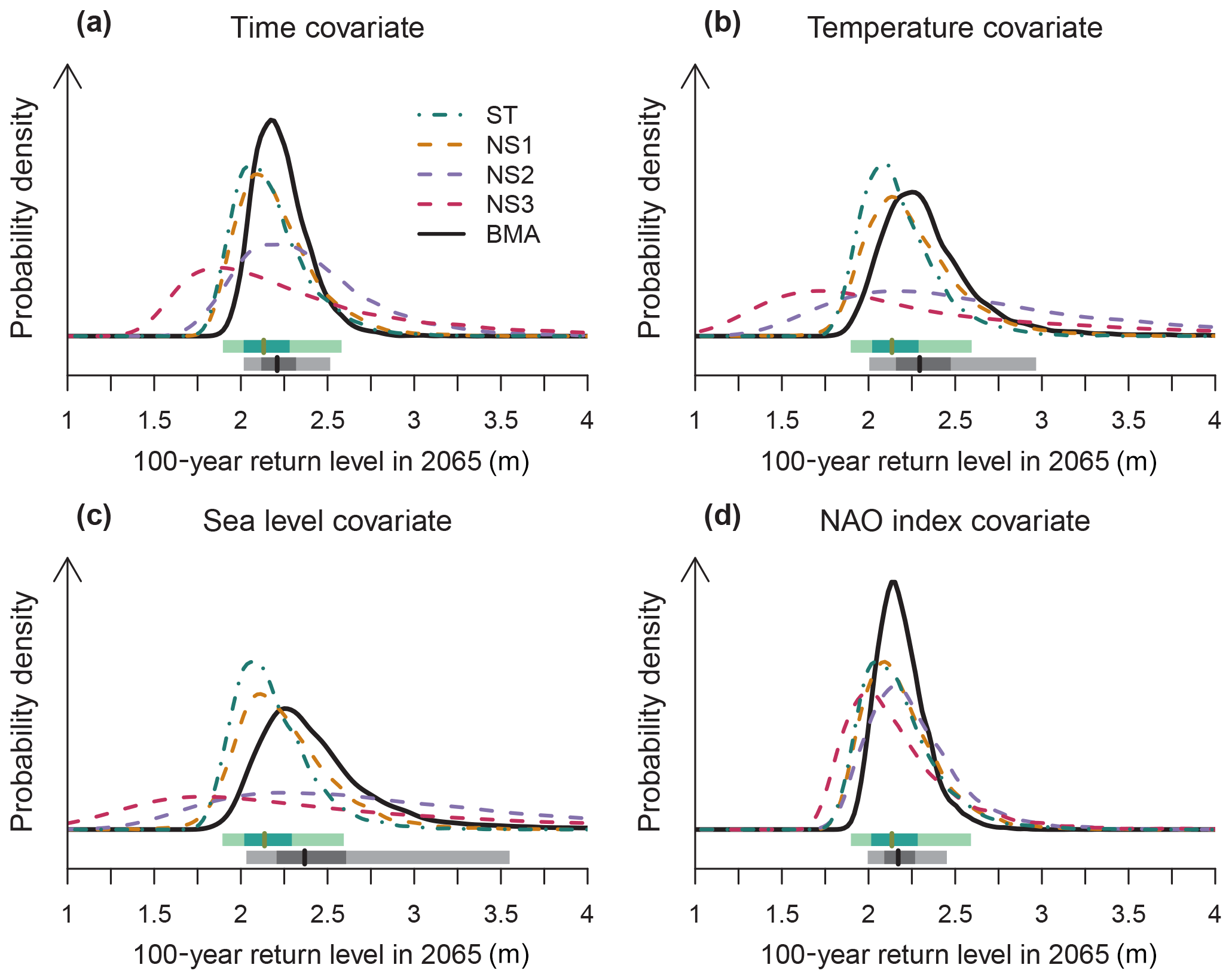
Figure 2 Empirical probability density functions for the 100-year storm surge return level (meters) at Norfolk, Virginia, as estimated using one of the four candidate model structures and using the Bayesian model averaging ensemble. Shown are nonstationary models where the statistical model parameters covary with (a) time, (b) global mean surface temperature, (c) global mean sea level and (d) winter mean NAO index. The bar plots provide the 5 %–95 % credible range (lightest shading), the interquartile range (moderate shading) and the ensemble medians (dark vertical line), for both the stationary model (green) and Bayesian model averaging ensemble (gray).

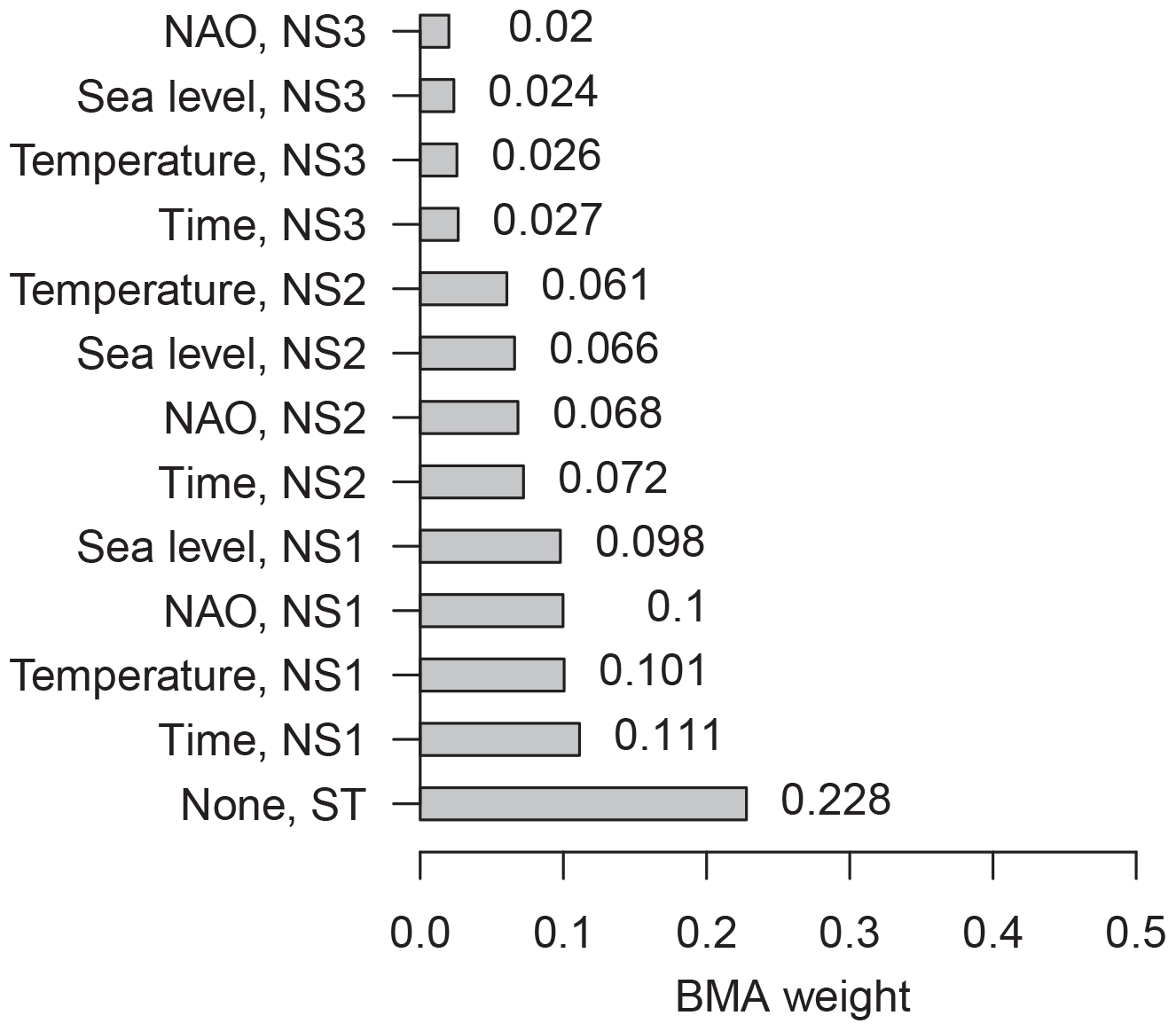
Figure 3 Bar plot showing the Bayesian model averaging weights for each of the 13 distinct candidate model structures, when all are simultaneously considered.

3.3 Integrating time-series information and across model structures

When all 13 distinct model structures are simultaneously considered in the BMA weighting, the models' BMA weights display a clear trend in favor of less-complex structures (Fig. 3). If one wishes to use these results to select a single model for projecting storm surge hazard, then, based on BMA weights, a stationary model would be the appropriate choice. In light of the results of Sect. 3.1, it is not surprising that the fully nonstationary models (NS3) are the poorest choices as measured by BMA weight. The models are assumed to all have uniform prior probability of 1∕13 (about 0.077). Therefore, these results indicate stronger evidence for the use of the stationary and NS1 models for modulating storm surges, and weaker evidence for incorporating nonstationarity in, for example, the GPD shape parameter (NS3).

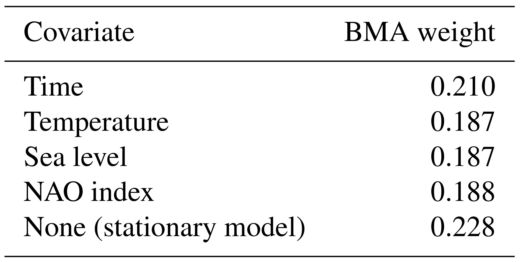
One interpretation of these results is that a stationary model (ST) receives about 23 % of the total model posterior probability, which is much more than the next largest BMA weight (about 10 %), so a stationary model is the “correct” choice. But an alternative and interesting question is raised: how important is each covariate, in consideration of all three nonstationary model structures (NS1-3)? A quantification of the total model posterior probability for each candidate covariate time series is given by adding up the BMA weights associated with each covariate's nonstationary models (Table 1). A stationary model still has the highest total BMA weight (0.23) but is followed closely by a simple linear change in PP/GPD parameters (0.21) as well as temperature, sea level and the NAO index (0.19). Taking this view, the fact that a stationary model has an underwhelming 23 % of the total model weight highlights the importance of accounting for the other 77 %, attributable to nonstationarity.

Table 1 Total BMA weight associated with each candidate covariate's nonstationary models and a stationary model (ST) for the full set of 13 candidate models, all considered simultaneously in the BMA weighting.

3.4 Accounting for more processes raises projected return levels

The BMA model that considers all of the covariate time series and levels of (non)stationarity has a median projected 2065 storm surge 100-year return level of 2.36 m (5 %–95 % credible range of 2.14 to 3.07 m; Fig. 4). This more detailed model has a higher central estimate (2.36 m) of flood hazard than all of the single-covariate models' BMA ensembles except for sea level (2.17 m for the NAO index, 2.21 m for time, 2.29 m for temperature and 2.37 m for sea level). When considering the set of multi-model, single-covariate BMA ensembles (Fig. 4, dashed colored lines) and the multi-model, multi-covariate BMA ensemble (Fig. 4, solid black line), there is a substantial amount of uncertainty in these projections of flood hazard attributable to model structure, in particular, with regard to the choice of covariate time series.

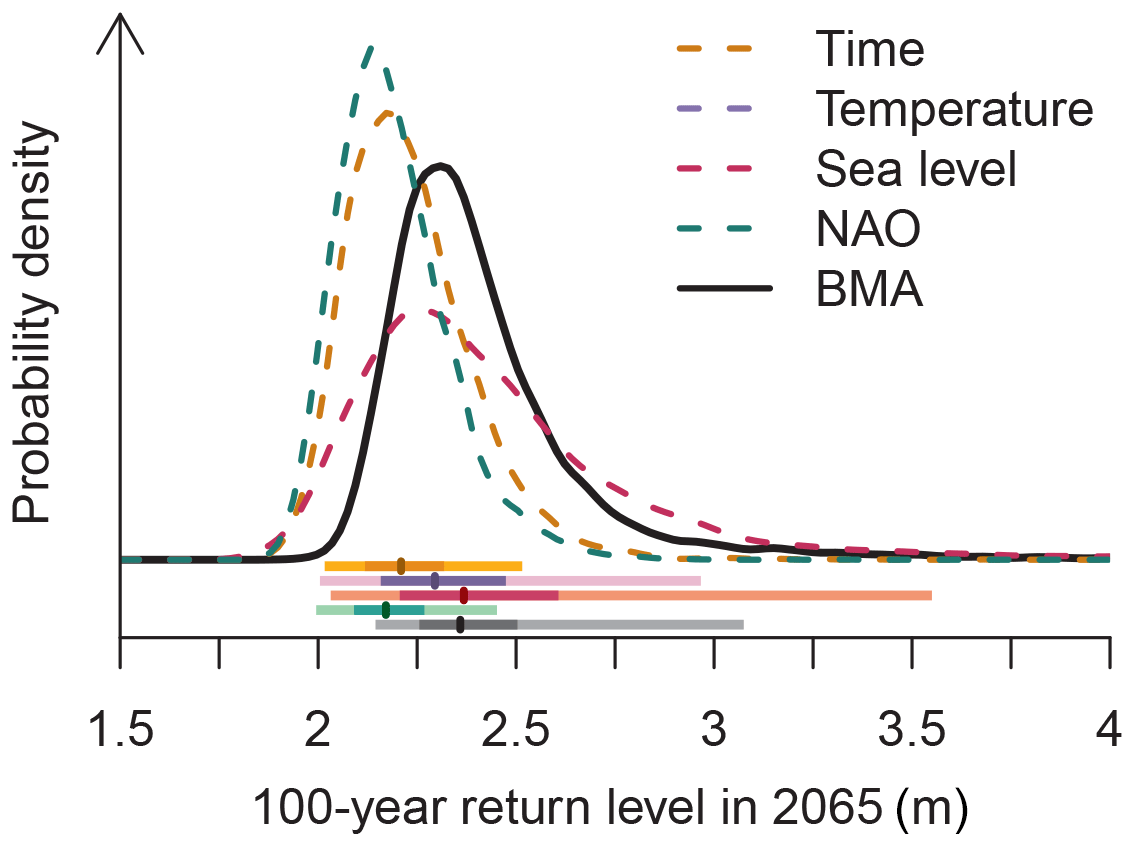
Figure 4 Empirical probability density functions for the 100-year storm surge return level (meters) at Norfolk, Virginia, as estimated using Bayesian model averaging with one of the four candidate covariates and using the overall Bayesian model averaging ensemble with all 13 distinct candidate model structures. The bar plots provide the 5 %–95 % credible range (lightest shading), the interquartile range (moderate shading) and the ensemble medians (dark vertical line). The shaded bar plots follow the same order as the legend.

4 Discussion

This study has presented and expanded upon an approach to integrate multiple streams of information to modulate storm surge statistical behavior (covariate time series) and to account for the fact that the “correct” model choice is almost always unknown. This approach improves the current status of storm surge statistical modeling by accounting for more processes (multiple covariates and model structures), thereby raising the upper tail of flood hazard (by up to 23 cm for Norfolk) while constraining these additional processes using BMA. These methods will be useful, for example, in rectifying disagreement between previous assessments using nonstationary statistical models for storm surges (e.g., Grinsted et al., 2013; Lee et al., 2017). The results presented here are consistent with those of Wong et al. (2018), who employed a single covariate BMA model based on the NAO index. Both studies demonstrate that the neglect of model structural uncertainties surrounding model choices leads to the underestimation of flood hazard.

These results are in agreement with the work of Lee et al. (2017) and highlight the importance of carefully considering the balance of model complexity against data availability. Including more complex physical mechanisms into model structures (i.e., nonstationary storm surges) is often important for decision-making, but additional model processes and parameters require more data to constrain them (Wong et al., 2018). If a single-model choice is to be made, then a stationary model may be the natural choice (Table 1). However, this work provides guidance on incorporating nonstationary processes to a degree informed by the model posterior probabilities, in light of the available data. Importantly, the (non)stationary model BMA weights were robust against the changes in the covariate time series used to modulate the storm surge model parameters (Fig. 1). By contrast, the largest uncertainty arises in the projections of flood hazard to 2065, depending on which covariate time series is used (Figs. 2 and 4). The primary contribution of this work is to present an approach to integrate across these covariate time series and overcome this issue of uncertainty in the “correct” covariate time series to use (Fig. 3). Using the stationary model leads to a distribution of the 100-year flood level with a median of 2.13 m and upper tail (95th percentile) of 2.58 m. Using the full multi-model, multi-covariate BMA model, however, substantially raises both the projected center (2.36 m) and upper tail (3.07 m) of the distribution of 100-year flood hazard in 2065, relative to using a stationary model. For Norfolk and the surrounding area, a difference of about 23 cm in the estimated return level can lead to millions of dollars in potential damages (Fugro Consultants, 2016). Thus, the present work also serves to demonstrate the potential risks associated with the selection of a single model structure.

Of course, some caveats accompany this analysis. The covariate time series are all deterministic model input. In particular, the temperature and sea level time series do not include the sizable uncertainties in projections of these time series, which in turn depend largely on deeply uncertain future emission pathways. The accounting and propagation of uncertainty and correlation in the covariate time series would be an interesting avenue for future study, but this is beyond the scope of this work. For example, temperature may drive changes in both sea levels and the NAO index, so future works might consider disentangling the effects of the multiple covariate time series. Furthermore, this study only considers derivatives of PP/GPD model structures and does not address the deep uncertainty surrounding the choice of statistical model (Wahl et al., 2017).

This study also focuses on a single tide-gauge station (Sewells Point in Norfolk, Virginia). This choice was made in light of the deep uncertainty surrounding how best to process and combine information across stations into a surge index (Lee et al., 2017) and because the Norfolk site is within the region studied by Grinsted et al. (2013), so the application of global mean surface temperature as a covariate is a reasonable extension of those authors' work. Extending these results to regions outside the southeastern part of the United States, however, is an important area for future study. A key strength of the fully nonstationary multi-covariate BMA model is that the methods presented here can be applied to any site, and the model posterior probabilities will allow the data to inform the weight placed on the different (non)stationary models and covariates, in light of the local tide-gauge information. As demonstrated by Grinsted et al. (2013), the use of local temperature or other covariate information may also lead to better constraint on storm surge return levels but also presents challenges for process models to reproduce potentially complex spatial patterns.

The present study is not intended to be the final word on model selection or projecting storm surge return levels. Rather, this work is intended to present a new approach for generating a model that accounts for more processes and modeling uncertainties and demonstrating its application to an important area for flood risk management. This study only presents a handful of many potentially useful covariates for storm surge statistical modeling (e.g., Grinsted et al., 2013). Future work should build on the methods presented here and can incorporate other mechanisms known to be important local climate drivers for specific applications.

5 Conclusions

This study has presented a case study for Norfolk, Virginia, that demonstrates the use of BMA to integrate flood hazard information across models of varying complexity (stationary versus nonstationary) and modulating model parameters using multiple covariate time series. This work finds that for the Norfolk site, all of the candidate covariates yield similar degrees of confidence in the (non)stationary model structures, and the overall BMA model that employs all four candidate covariates projects a higher flood hazard in 2065. These results provide guidance on how best to incorporate nonstationary processes into flood hazard projections, and a framework to integrate other locally important climate variables, to better inform coastal risk management practices.

Appendix A

Table A1 CMIP5 models employed in the present study.

Table A2 Quantiles of the estimated storm surge return levels (meters) for Norfolk (Sewells Point) in 2065 using the full nonstationary multi-covariate BMA model.

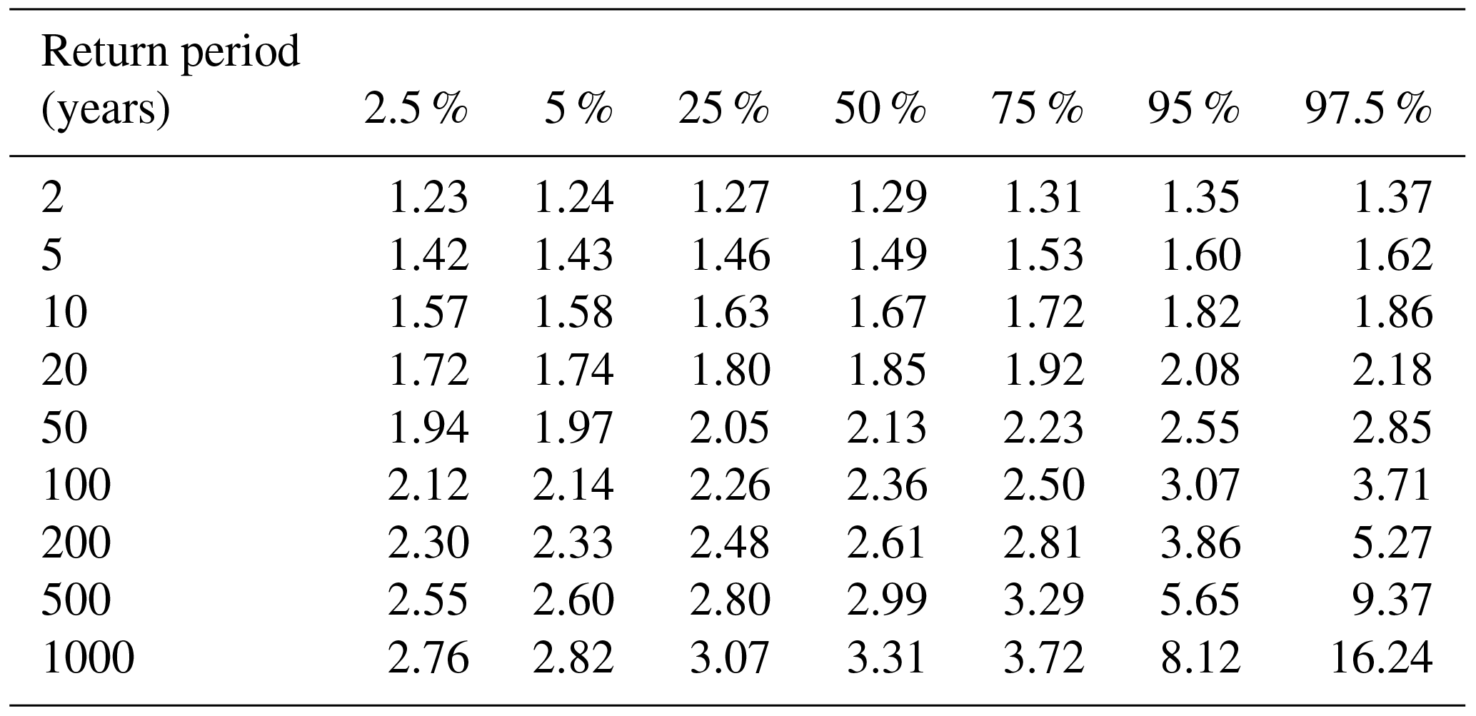
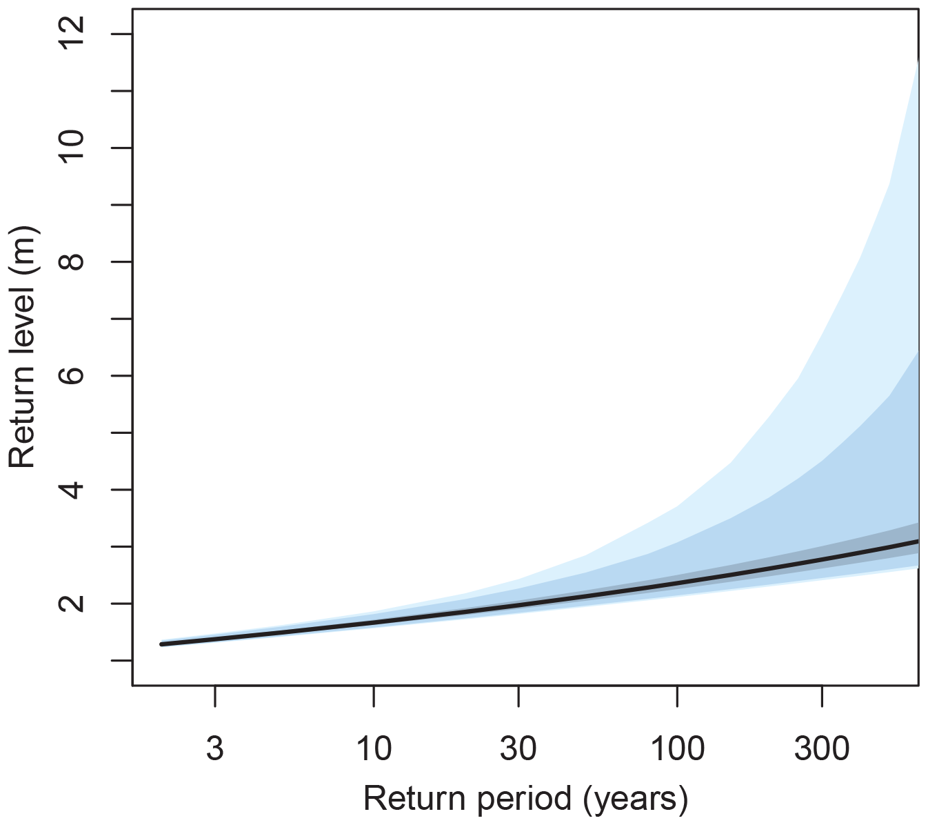
Figure A1 Storm surge return periods (years) and associated return levels (meters) in 2065 for Norfolk, using the full nonstationary multi-covariate BMA model. The solid line indicates the ensemble median, the darkest shaded region denotes the 25th–75th percentile range, the medium shaded region denotes the 5th–95th percentile range and the lightest shaded region denotes the 2.5th–97.5th percentile range.