the Creative Commons Attribution 3.0 License.
the Creative Commons Attribution 3.0 License.
An improved projection of climate observations for detection and attribution
Alexis Hannart
An important goal of climate research is to determine the causal contribution of human activity to observed changes in the climate system. Methodologically speaking, most climatic causal studies to date have been formulating attribution as a linear regression inference problem. Under this formulation, the inference is often obtained by using the generalized least squares (GLS) estimator after projecting the data on the r leading eigenvectors of the covariance associated with internal variability, which are evaluated from numerical climate models. In this paper, we revisit the problem of obtaining a GLS estimator adapted to this particular situation, in which only the leading eigenvectors of the noise's covariance are assumed to be known. After noting that the eigenvectors associated with the lowest eigenvalues are in general more valuable for inference purposes, we introduce an alternative estimator. Our proposed estimator is shown to outperform the conventional estimator, when using a simulation test bed that represents the 20th century temperature evolution.
- Article
(2153 KB) - Full-text XML
- BibTeX
- EndNote


1.1 Context
An important goal of climate research is to determine the causes of past global warming in general and the responsibility of human activity in particular (Hegerl et al., 2007); this question has thus emerged as a research topic known as detection and attribution (D&A). From a methodological standpoint, D&A studies are usually based on linear regression methods, often referred to in this particular context as optimal fingerprinting, whereby an observed climate change is regarded as a linear combination of several externally forced signals added to internal climate variability (Hasselmann, 1979; Bell, 1986; North et al., 1982; Allen and Tett, 1999; Hegerl and Zwiers, 2011). On the one hand, the latter signals consist of spatial, temporal or space–time patterns of response to external forcings as anticipated by one or several climate models. Internal climate variability, on the other hand, is usually represented by a centred multivariate Gaussian noise. Its covariance Σ, which is also estimated from model simulations, thus describes the detailed space–time features of internal variability. In particular, its eigenvectors can often be interpreted as the modes of variability, whose relative magnitudes are reflected by the associated eigenvalues.
Denoting y the n-dimensional vector of observed climate change, the n×p matrix concatenating the p externally forced signals and ν the internal climate variability noise, the regression equation is as follows:
The results of the inference on the vector of regression coefficients β, and the magnitude of its confidence intervals, determine whether the external signals “are present in the observations” (Hegerl and Zwiers, 2011) and whether or not the observed change is attributable to each forcing.
Under the assumption that Σ is known, the above inference problem can be solved using the standard generalized least squares (GLS) setting (e.g. Amemiya, 1985). Under this framework, the expression of the best linear unbiased estimator (BLUE) and its variance are given by the following:
The GLS estimator of Eq. (2) can be obtained as the ordinary least squares (OLS) estimator for the linearly transformed regression equation:
where the n×n transformation matrix T is such that the components of the transformed noise Tν are independent and identically distributed (IID). This condition yields and an admissible choice for T is thus as follows:
where with is the matrix of eigenvalues of Σ and is its matrix of column eigenvectors, i.e. . In Eq. (3), the data are thus projected on the eigenvectors of the covariance matrix scaled by the inverse square root of their eigenvalues.
In most applications, the covariance Σ is not known and Eq. (2) cannot be implemented. This has given rise to many theoretical developments (e.g. Poloni and Sbrana, 2014; Naderahmadian et al., 2015) which often rely on further assumptions regarding the covariance Σ, in order to allow for its estimation simultaneously with β. In the applicative context of D&A considered here, the situation may be viewed as an in-between between known and unknown Σ because we have access to an ensemble of unforced climate model simulations. This ensemble can be used to extract valuable information about Σ. However, the resulting knowledge of Σ is imperfect for two reasons. First, the size of the ensemble is often very small, typically a few dozens, because of the high cost of numerical experiments requiring intensive computational resources. For the range of dimensions n usually considered, typically a few hundreds or thousands, the empirical covariance S may thus be non-invertible. Second, climate model simulations are known to inadequately represent the modes of internal variability at the smaller scale. Those smaller scale modes have lower magnitude and are expected to be associated with eigenvectors with low eigenvalues. Furthermore, the latter eigenvectors with low eigenvalues are also poorly sampled by construction and therefore are difficult to estimate reliably (North et al., 1982). For these two reasons, it is often assumed that only a small number r of leading eigenvectors of Σ, which are denoted and r is typically on the order of 10, can be estimated from the control runs with enough reliability. Accordingly, it is assumed that the remaining n−r eigenvectors and eigenvalues are unknown.
Under this assumption, the inference on β must therefore be obtained based on these r leading eigenvectors only. The conventional approach presently used in D&A studies to tackle this problem follows from a simple and straightforward idea: adapting Eq. (4) to this situation by restricting the image of the transformation matrix T to the subspace generated by the r leading eigenvectors, thus leading to a truncated transformation having the following expression:
where and . A new estimator thus follows by similarly applying the OLS estimator to the transformed data (Trx,Try):
where is the pseudo-inverse of . Finally, from a mere terminology standpoint, applying the truncated transformation Tr to the data is often referred to in D&A as “projecting” the data onto the subspace spanned by the leading eigenvectors. However, Tr is in fact not a projection from a mathematical standpoint insofar as hence we prefer to use the word “transformation”.
1.2 Objectives
The solution recalled above in Eq. (6) is easy to use and may seem to be a natural choice. It emerged as a popular approach in D&A arguably for these reasons. Nevertheless, this approach has two important limitations. Firstly, as pointed out by Hegerl et al. (1996), the leading eigenvectors sometimes fail to capture the signals x. Indeed, the leading eigenvectors capture variability well, but not necessarily the signal, merely because the corresponding physical processes may differ and be associated with different patterns. Secondly, by construction, the subspace spanned by the leading eigenvectors maximizes the amplitude of the noise, thereby minimizing the ratio of signal to noise and affecting the performance of the inference on β.
The first objective of this article is to highlight in detail these two limitations: both will be formalized and discussed immediately below in Sect. 2. Its second objective is to circumvent these limitations by building a new estimator of β that performs better than the conventional estimator of Eq. (6) while still making the same assumptions and using the same data. Most importantly, the central assumption here is that only the r leading eigenvectors of Σ can be estimated with enough accuracy from the control runs. Furthermore, we assume that r is given and is small compared to n (e.g. r is on the order of 10), and that N control runs are available to estimate the r leading eigenvectors with N≥r.
Section 2 highlights the limitations of the conventional estimator . Section 3 introduces our proposed estimator . Section 4 evaluates the benefit of our approach based on a realistic test bed, and illustrates it on actual observations of surface temperature. Section 5 concludes the paper.
2.1 General considerations
It is useful to start this discussion by returning for a moment to the case where Σ is assumed to be fully known, i.e. its n eigenvectors are all known perfectly, as well as their eigenvalues. Under this assumption, let us evaluate the benefit of a given eigenvector vk, , for the inference of β. For this purpose, we propose to compare the variance of the BLUE estimator of Eq. (2) obtained by using the transformation matrix , to the variance of the estimator obtained by using the transformation matrix where V−k and Δ−k exclude the kth eigenvector and the kth eigenvalue respectively. From Eq. (2), these variances can be rewritten after some algebra:
The Sherman–Morrison–Woodbury formula is a well known formula in linear algebra, which shows that the inverse of a rank-one correction of some matrix, can be conveniently computed by doing a rank one correction to the inverse of the original matrix. By applying the Sherman–Morrison–Woodbury formula to Eq. (7), we obtain the following:
Unsurprisingly, an immediate implication of Eq. (8) is that removing any eigenvector vk results in an increase of the variance of the estimator. Indeed, the matrix in the second term of the right-hand side of Eq. (8) is positive definite; it can thus be interpreted as the cost in variance increase of excluding vk or conversely as the benefit in variance reduction of including vk. Moreover, the most valuable eigenvectors for inferring β in the above-defined sense are those combining a small eigenvalue (low λk) and a good alignment with the signals x (high x′vk). Accordingly, for any eigenvector vk, its benefit is a decreasing function of λk, everything else being constant.
A similar conclusion can be reached by using a different approach. Consider this time the transformation . Since T* is a p×n matrix, the data dimension is thus drastically reduced from n to p in the transformed Eq. (3). Furthermore, noting that the noise components T*ν have covariance , and applying the GLS estimator to the transformed data , we obtain an estimator which has the following expression:
After some algebra, the above expression of simplifies to the following:
which is exactly the expression of the estimator of Eq. (2). Therefore, remarkably, the BLUE estimator obtained from the full data (y,x) is entirely recovered from the transformed data when using the subspace spanned by T*. The latter subspace can thus be considered as optimal, in the sense that it reduces the data dimension to its bare minimum p while still preserving all the available information for inferring β. The p directions of the subspace spanned by T* are denoted . They have the following expression:
Consistently with Eq. (8), Eq. (11) shows that for each , the optimal direction emphasizes the eigenvectors that best trade off the smallest possible eigenvalue (i.e. small noise) with the best possible alignment between the eigenvector and the signal xk (i.e. strong signal). It is interesting to notice that the foremost importance of small eigenvalues, which is underlined here, is also quite obvious in the formulation of optimal detection proposed by North and Stevens (1998). However, the importance of small eigenvalues was lost later on, as truncation on leading eigenvectors became a popular practice.
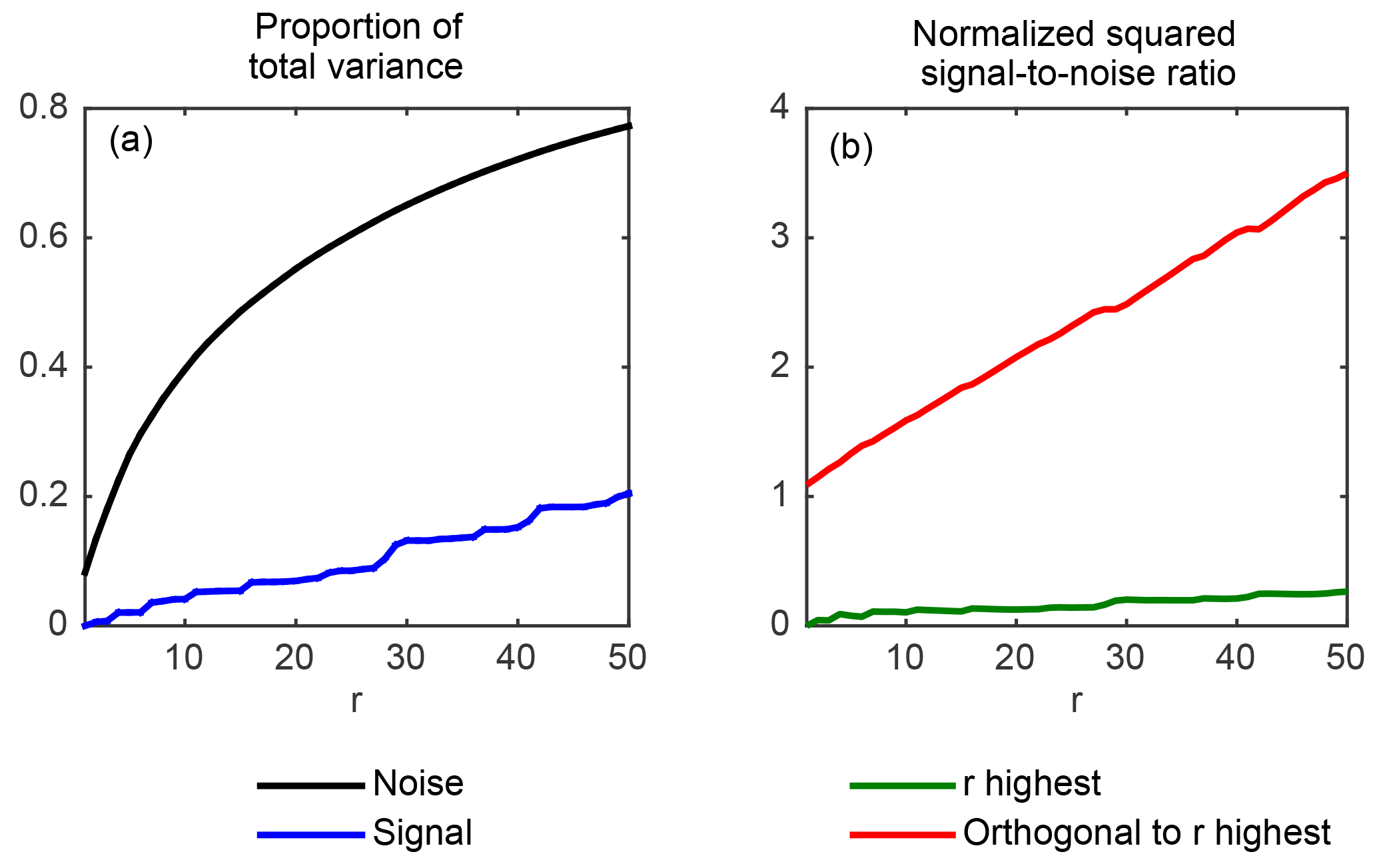
Figure 1(a) Proportion of the total variance of the projected anthropogenic signal (thick blue line) and of the projected noise (thick black line) as functions of r; uniform increase r∕n (light black line). (b) Signal-to-noise ratio of the projected data when using the projection subspace Vr consisting of the r leading eigenvectors (thick green line) and when using the orthogonal subspace (thick red line) as functions of r. Both values are normalized to the signal-to-noise ratio of the full data.
In light of these considerations, the two main limitations of the conventional estimator of Eq. (6), mentioned in Sect. 1, appear more clearly. Firstly, in agreement with Hegerl et al. (1996), there is no guarantee that the leading eigenvectors will align well with the signals at stake. Secondly, the leading eigenvectors are by definition those with the largest eigenvalues. Therefore, a straightforward truncation onto the leading eigenvectors, such as the one used in , maximizes the noise instead of minimizing it. While the first limitation may be an important pitfall in some cases, it will not be an issue whenever the signals align well with the leading eigenvectors, which nothing prevents in general. In contrast, the second limitation always manifests whenever is used and is thus arguably a more serious problem of the conventional approach. In the present paper, we thus choose to focus restrictively on this second limitation, and to not address the first one.
2.2 Illustration
In order to illustrate the second issue more concretely, we use surface temperature data from Ribes and Terray (2012), described in more detail in Section 4. The signals x considered here consist of the responses to anthropogenic and natural forcings, with p=2 and n=275. Both x and the covariance Σ are obtained from climate model simulations. The r leading eigenvectors are obtained from Σ and are assumed to be known. The proportion of the noise's total variance retained by projecting the data on Vr is denoted while the proportion of the signal's total variance associated with the same projection is denoted . Since the projection matrix associated with projecting on the subspace Vr is equal to VrVr′, we have the following:
where for any vector z, denotes the empirical variance of z. Figure 1a plots and computed from Eq. (12) applied to the above-mentioned data. For simplicity, is shown only for the anthropogenic signal x1. As expected from the expression of given in Eq. (12), it can be seen from this plot that increases with r much faster than r∕n, since by definition the leading eigenvectors concentrate most of the noise's variance. In contrast, increases with r roughly like r∕n: this shows that, in this example, the signal projects nearly uniformly on each eigenvector. For instance, when r=20, Vr involves 7 % of the n eigenvectors, and accordingly, projecting on Vr retains 8 % of the signal's total variance. In contrast, as much as 55 % of the noise's total variance is retained by projecting on Vr. Consequently, the signal-to-noise ratio of the projected data (see Fig. 1b) is reduced by a factor of 7 compared to the signal-to-noise ratio of the full data. Hence, it is fair to say that, in this case, the projection on the leading eigenvectors is greatly suboptimal, insofar as it drastically reduces the signal-to-noise ratio.
Let us now consider the quantities and defined as above, but projecting this time on the subspace orthogonal to Vr. By construction,
As a direct consequence, for r=20, the projection on the subspace orthogonal to Vr captures 92 % = 100 %–8 % of the total variance of the signal, while the variance of the projected noise is only 20 % = 100 %–80 % of the total. Therefore, the signal-to-noise ratio of the projected data (see Fig. 1b) is this time magnified by a factor of 2 compared to the signal-to-noise ratio of the full data, and by a factor of 14 when comparing to the signal-to-noise ratio of the data projected on Vr. It can thus be seen that projecting the data on the orthogonal to Vr greatly magnifies the signal-to-noise ratio by filtering out a large fraction of the noise, while retaining most of the signal. These characteristics arguably make it a much more relevant projection subspace for the purpose of estimating β than the subspace of the leading eigenvectors. We further elaborate on this idea in Sect. 3.
3.1 Description
With these preliminary considerations in hand, we return to the situation of direct interest here: inferring β when only the r leading eigenvectors are available. In an attempt to improve the conventional estimator , we propose the following new estimator:
Like the conventional estimator , the proposed estimator only uses the data (y,x) and the r leading eigenvectors . Its formulation stems from the above considerations regarding the suboptimality of the subspace Tr of Eq. (5) spanned by the leading eigenvectors, as we now highlight.
Let us denote a matrix consisting of n−r orthonormal column vectors spanning the subspace orthogonal to . In other words, we have the following by construction:
Note that infinitely many matrices satisfy Eq. (16), and that it is straightforward to construct one such matrix from the r leading eigenvectors , for instance by using the Gram–Schmidt algorithm. Furthermore, it is also important to note that, since is orthogonal to Vr, it spans the same subspace as the subspace spanned by the n−r eigenvectors associated with the smallest eigenvalues, because the latter are also orthogonal to by definition. Therefore, it is not necessary to have knowledge of these n−r eigenvectors in order to be able to project the data onto the latter subspace: only the knowledge of is required for that purpose. Thus, with the knowledge of the r leading eigenvectors only, we are able to project the data onto the orthogonal subspace spanned by using the transformation matrix , thus obtaining . The estimator proposed in Eq. (15) consists of using the OLS estimator corresponding to these transformed data:
It is interesting to note that the orthogonal projection subspace does not actually need to be obtained to derive because only matters for this purpose, and this matrix happens to be directly known from Vr through the orthogonality Eq. (16). This yields the right-most term of Eq. (17), which corresponds to the expression of given above in Eq. (15).
However, the choice of applying the OLS estimator to the projected data as implied by Eq. (17), rather than applying the GLS estimator, may seem surprising at first. The rationale for this choice is the following. Since we only assume knowledge of the r leading eigenvectors, the projection subspace is thus by construction unknown from the standpoint of the covariance of the projected noise. In other words, while the projected noise in the projected regression equation remains Gaussian centred, we do not know anything about its covariance. Thus, we use by default the assumption that is IID with unknown variance σ2, which is a commonplace assumption used in regression analysis when nothing is known about the noise's covariance. An immediate implication of this assumption is that the associated log likelihood is the following:
The complete likelihood of Eq. (18) can be concentrated in β by maximizing out σ2 to obtain the concentrated likelihood ℓc(β):
Our proposed OLS estimator results from the maximization of the above likelihood. The above considerations also have some implications with respect to the uncertainty analysis on the proposed estimator . Indeed, in the present context, it is straightforward to obtain confidence intervals around based on the ratio of likelihoods , following a classic approach in statistics that is often used in D&A (e.g. Hannart et al., 2014).
It is important to underline that the latter approach to uncertainty quantification relies on the assumption that the projected noise is IID. Since the unknown true covariance of is in fact equal to , this assumption is incorrect and hence the resulting confidence intervals are prone to be incorrect as well. An initial assessment under test bed conditions described in Section 4 suggested that the proposed approach is conservative in the sense that it leads to an overestimation of uncertainty (not shown). However, a more detailed assessment of the performance of this uncertainty quantification procedure is needed, but is beyond the scope of the present paper.
3.2 Extension to total least squares
The signals x are estimated as the empirical averages of several ensembles of finite size m, which introduces sampling uncertainty. In order to account for the latter, it is commonplace in D&A to reformulate the linear regression model of Eq. (1) as an error-in-variables (EIV) model (Allen and Stott, 2003):
where x* is now an unobserved latent variable, x is the ensemble average estimator of the true responses x* and ε is a Gaussian centred noise term with covariance Σ∕m.
It is straightforward to generalize the approach exposed in Sect. 2.3 to this error-in-variables regression model. Likewise, the data (y,x), the latent variable x*, and the noise terms ν and ε are projected on the orthogonal subspace using . The projected residuals are then also assumed IID with unknown variance σ2. This yields the following complete likelihood:
which can be concentrated in β by maximizing out σ2 and x* to obtain the concentrated likelihood ℓc(β):
The so-called total least squares (TLS) estimator results from the maximization of the above concentrated likelihood in β, and is available under a closed form expression:
where is a p-dimensional vector and zp+1 is a scalar, such that is the eigenvector associated with the smallest eigenvalue of the positive definite matrix of size p+1. The estimator of Eq. (23) is a generalization of the OLS estimator of Eq. (17), the latter is indeed a special case of the former for . Furthermore, in the particular case p=1 which is often referred to as the Deming regression, the estimator of Eq. (23) takes the following expression:
where , and . Next, following the same approach as in Sect. 2.3, it would be tempting to derive confidence intervals around based on the ratio of likelihoods . While this approach performs reasonably well in the context of EIV regression with known variance (Hannart et al., 2014), it is known to be problematic in the present context of EIV regression with unknown variance (Casella and Berger, 2008; Sect. 12.2). In this case, more suitable alternatives are available, e.g. an estimator of the variance of for p=1 is given by Fuller (1987) Sect. 1.3; it has the following expression:
from which confidence intervals can be obtained. When p > 1 the above variance estimator is applied successively to each component i of () by replacing y with in Eq. (25). It is worthwhile noting that various approaches are available in the literature to tackle the general problem of deriving confidence intervals for β under the present EIV regression model with unknown variance. While it would be worthwhile to investigate and to compare their performance in practice in a D&A context, such investigation is beyond the scope of this paper.
Summarizing, the proposed solution here to deal with the case of error in variables thus consists of using Eq. (23) to derive an estimate of β and Eq. (25) to derive a confidence interval.
3.3 Continuity considerations
The motivation of this subsection is merely to provide a more in-depth mathematical grounding to the proposed estimator, beyond the general considerations of Sect. 2.1. This subsection can safely be skipped without affecting the understanding of the remainder of this article, in so far as it does not provide any additional results or properties regarding the estimator itself.
The idea here is that, in addition to the general considerations of Sect. 2.1, the proposed estimator can also be justified by following a continuity extension argument. For any given x and y, let us consider the BLUE estimator of Eq. (2) as a function of the known covariance Σ. For this purpose, we define the function f on the set of positive definite matrices of dimension n, denoted , as follows:
so that we have .
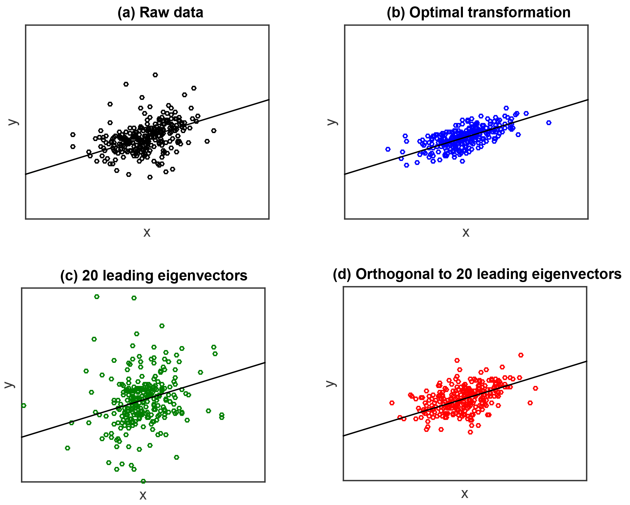
Figure 2(a) Scatter plot of one realization of the raw data (y,x) using the simulation test bed of Section 4: the observation vector y is plotted on the vertical axis and the first column vector x1 of the matrix x is plotted on the horizontal axis. (b) Same as (a) for the transformed data Ty and Tx using the optimal transformation matrix . (c) Same as (b) when using the truncated transformation matrix on the leading eigenvectors, with r=20. (d) Same as (b) when using the proposed transformation matrix with r=20.
In the present context, we assumed that Σ is unknown but that is known. While it is tempting to apply f in Σr, unfortunately Σr is not positive definite so that f is not defined in Σr. Hence, an estimate of β cannot be obtained by straightforwardly applying the function f in Σr. Nevertheless, Σr belongs to the set of positive semi-definite matrices, denoted , which has the following interesting topological property:
where for any subset E, the notation used above in Eq. (27) denotes the adherence of E. Equation (27) thus implies that is dense in , which means that for any positive semi-definite matrix A there exists a sequence of positive definite matrices converging to A. Equation (27) therefore suggests the possibility to define a function which continuously extends f to the set of positive semi-definite matrices. For this purpose, let us consider the matrix A+εI with ε>0. It is immediate to show that for any and for any arbitrarily small but positive ε, we have . Taking advantage of this remark, we define by . With this definition, can be obtained under a closed form expression:
The proof of Eq. (28) is detailed in Appendix A. The proposed estimator of Eq. (15) is therefore obtained by applying the extended function defined above, to the known, positive semi-definite matrix Σr:
4.1 Data
We illustrate the method by applying it to surface temperature data and climate model simulations over the 1901–2000 period and over the entire surface of the Earth. For this purpose, we use the data described and studied in Ribes and Terray (2012). The temperature observations are based on the HadCRUT3 merged land–sea temperature data set (Brohan et al., 2006). The simulated temperature data used to estimate the response patterns are provided by results from the CMIP5 archive arising from simulations performed with the CNRM-CM5 model of Météo France under NAT and ANT experiments. For both experiments, the size of the ensembles is m=6. However, estimates of internal variability are based on intra-ensemble variability from 10 CMIP5 models (CNRM-CM5, CanESM2, HadGEM2-ES, GISS-E2-R, GISS-E2-H, CSIRO-Mk3-6-0, IPSL-CM5A-LR, BCC-CSM1-1, NorESM1-M, FGOALS-g2) under NAT and ANT experiments as well as pre-industrial simulations from both the CMIP3 and CMIP5 archives, leading to a large ensemble of 374 members. Standard pre-processing is applied to all observed and simulated data. Data are first interpolated on the 5∘ × 5∘ observational grid and then the spatio-temporal observational mask is applied. The dimension of the data set is then further reduced by computing decadal means and projecting the resulting spatial patterns onto spherical harmonics with resolution T4 to obtain vectors of size n=275 (see Ribes et al., 2012 for more details about ensembles and pre-processing). The ANT and NAT individual responses (p=2) are estimated by averaging the corresponding two ensembles to obtain the matrix of regressors x. The covariance matrix Σ is estimated as the empirical covariance of the large ensemble of control runs.
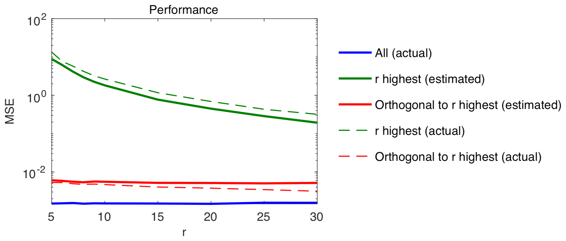
Figure 3Performance results on simulated data: MSE of several estimators of β (vertical axis) as functions of the number of eigenvectors r (horizontal axis) assumed to be reliably estimable from control runs: conventional estimator computed based on estimated eigenvectors (thick green line) with N=30, and based on the true eigenvectors (light green line); proposed orthogonal estimator computed based on estimated eigenvectors (thick red line) with N=30, and based on the true eigenvectors (light red line); GLS estimator computed based on the true value of the covariance Σ (thick blue line).
4.2 Performance on simulated data
This section evaluates the performance of the estimators described above, by applying it to simulated values of y obtained from the linear regression equation assumed by the model of Eq. (1), where the noise ν is simulated from a multivariate Gaussian distribution with covariance Σ and where is used. This setting thus assumes that x is known exactly, therefore it does not include the EIV situation prevailing in Eq. (20) and in Sect. 3.3 where x is measured with an error.
The use of simulated rather than real data aims at verifying that our proposed estimator performs correctly, and at comparing its performance with the conventional procedure, a goal which requires the actual values of β to be known. A sample of N=30 control runs was also simulated from a multivariate Gaussian distribution with covariance Σ, and the r leading eigenvectors and eigenvalues were estimated from these control runs.
Figure 2 shows scatter plots of one realization of the data (x,y) under this test bed, for the raw data (x,y) as well as for the transformed data (Tx,Ty), when using the three main transformations considered above: the optimal transformation which assumes a fully known covariance Σ; the truncated transformation matrix on the r leading eigenvectors, with r=20, and the proposed projection matrix on the orthogonal to the r leading eigenvectors, again with r=20. Figure 2 allows the behavior of these transformations to be visualized. Firstly, the benefit of the optimal transformation appears clearly, as it greatly enhances the signal. Secondly, it is also apparent that the standard truncated transformation using the r leading eigenvectors fails to enhance the signal, actually leading to a cloud of points which is more noisy than the original raw data. In contrast, the proposed transformation on the orthogonal to the r leading eigenvectors accurately captures part of the signal enhancement produced by the optimal transformation.

Figure 4Illustration of temperature data with r=20. (a) Regression coefficients βANT and βNAT estimated using the conventional estimator : value of the estimate (green dots) and 95 % confidence interval (thick black lines). (b) Same as (a) under the proposed estimator .
The conventional estimator and the proposed estimator of Eq. (15) were both derived based on the r leading estimators estimated from the N control runs. Then, these two estimators were derived again, this time using the true values of the r leading eigenvectors, for comparison. Finally, the GLS estimator of Equation (1) was derived based on the true value of the covariance Σ. The performance of each five estimators of β thus obtained was evaluated based on average mean squared error (MSE) , where denotes the simulation number and J=1e4. These calculations were repeated for several values of r ranging from 5 to 30. Results are plotted in Fig. 3. They show an important gap in MSE between the proposed estimator and the conventional approach with the former exceeding the latter by a factor of 1000 for r=5, decreasing to 80 for r=30. This gap suggests a substantial benefit of using and strongly emphasizes the relevance of this approach compared to the conventional one.
When comparing the performance of using estimated vs. actual values of the r leading eigenvectors, a slight benefit of using actual values is found. This benefit increases with r, as eigenvectors with lower eigenvalues tend to be more difficult to estimate. In contrast, when comparing the performance of using estimated vs. actual values of the r leading eigenvectors, a slight benefit of using the estimated values is found. This superiority of the estimated, and thus incorrect, values may seem surprising at first, but is in fact natural and in line with our main point. Indeed, it can be explained by the fact that the estimated leading eigenvectors match to a large extent with Vr but also span to some extent the true orthogonal subspace , which, according to our main point here, is much more suited for estimating β. Unsurprisingly, the estimator based on the estimated leading eigenvectors thus performs better than its counterpart based on actual values.
4.3 Illustration on real data
The method is finally illustrated by applying it to actual observations of surface temperature y, with the same regressors x and covariance Σ as described above. The observed temperature data y is based on the HadCRUT3 merged land–sea temperature data set (Brohan et al., 2006). The method is applied for r=20. Further, we use a number of control runs N that is small compared to n, which is a common situation, even though we have access under the present test bed to 374 control runs. Thus, N=30 control runs are randomly selected from the 374 control runs available and the eigenvectors are estimated from these 30 runs. For the inference of β and confidence intervals, we use the solution described in Sect. 3.2 which consists of using Eq. (23) to derive an estimate of β and Eq. (25) to derive a confidence interval. Results are shown in Fig. 4. For the scaling factor corresponding to anthropogenic forcings, both methods yield an estimate which is close to 1 and significantly positive. However, the level of uncertainty obtained with the proposed estimator is 3 times smaller than when using the conventional method. An even wider uncertainty gap is observed for the coefficient corresponding to natural forcings. In this case, the confidence interval includes zero under the conventional approach, but it does not under the proposed orthogonal approach. However, as already stated in Sect. 3, a caveat in the latter result is that the uncertainty quantification procedure used here has not been evaluated in detail, and thus we do not know for sure that the obtained uncertainty estimate is well calibrated.
We have introduced a new estimator of the vector β of linear regression coefficients, adapted to the context where only the r leading eigenvectors of the noise's covariance Σ are known, which is an assumption often relevant in climate change attribution studies. General considerations have first shown that when the covariance is known, its most relevant eigenvectors for projection are those trading off the smallest possible eigenvalue with the best possible alignment to the signal. The optimal direction is thus associated in general with the smallest eigenvalues, not with the highest ones. Our proposed estimator builds upon this finding and is based on projecting the data on a subspace which is orthogonal to the r leading eigenvectors.
When applied on a simulation test bed that is realistic with respect to D&A applications, we find that the proposed estimator outperforms the conventional estimator by several orders of magnitude for small values of r. Our proposal is thus prone to significantly affect D&A results by decreasing the estimated level of uncertainty.
Substantial further work is needed to evaluate the performance of the proposed uncertainty quantification, in particular in an EIV context. Such an evaluation was beyond the scope of the present work. Its primary focus was to demonstrate that the choice of the leading eigenvectors as a projection subspace is a vastly suboptimal one for D&A purposes; and that projecting on a subspace which is orthogonal to the r leading eigenvectors yields a significant improvement.
The data used for illustration throughout this article was first described and studied by Ribes and Terray (2013). As mentioned in the latter study, it can be accessed at the following url: http://www.cnrm-game.fr/spip.php?article23&lang=en (last access: 19 December 2018).
Let be a non-invertible positive matrix. Denote ΔA the matrix of non-zero eigenvalues of A, VA the matrix of eigenvectors associated with ΔA and the matrix of eigenvectors associated with the eigenvalue zero. For ε>0, we have the following:
Therefore,
with . We have , hence,
which proves Eq. (28).
The author declares that there is no conflict of interest.
This work was supported by the ANR grant DADA and by the LEFE grant MESDA. I
thank Dáithí Stone, Philippe Naveau and two anonymous reviewers for very
useful comments and discussions that helped improve considerably this
article.
Edited by: Christopher Paciorek
Reviewed by: two anonymous referees
Allen, M. and Stott, P.: Estimating signal amplitudes in optimal fingerprinting, part i: theory, Clim. Dynam., 21, 477–491, 2003. a
Allen, M. and Tett, S.: Checking for model consistency in optimal fingerprinting, Clim. Dynam., 15, 419–434, 1999. a
Amemiya, T.: Advanced Econometrics, Harvard University Press, 1985. a
Bell, T. P.: Theory of optimal weighting of data to detect climate change, J. Atmos. Sci., 43, 1694–1710, 1986. a
Brohan, P., Kennedy, J., Harris, I., Tett, S., and Jones, P.: Uncertainty estimates in regional and global observed temperature changes: a new data set from 1850, J. Geophys. Res., 111, D12106, https://doi.org/10.1029/2005JD006548, 2006. a, b
Casella, G. and Berger, R. L.: Statistical Inference, Duxbury, 2nd Edition, 2008. a
Fuller, W. A.: Measurement Error Models, John Wiley, New York, 1987. a
Hannart, A.: Integrated Optimal Fingerprinting: Method description and illustration, J. Climate, 29, 1977–1998, 2016.
Hannart, A., Ribes, A., and Naveau, P.: Optimal fingerprinting under multiple sources of uncertainty, Geophys. Res. Lett., 41, 1261–1268, https://doi.org/10.1002/2013GL058653, 2014. a, b
Hasselmann, K.: On the signal-to-noise problem in atmospheric response studies, in: Meteorology of tropical oceans, edited by: Shaw, D. B., 251–259, Royal Meteorological Society, London, 1979. a
Hegerl, G. C. and North, G. R.: Comparison of statistically optimal methods for detecting anthropogenic climate change, J. Climate, 10, 1125–1133, 1997.
Hegerl, G. and Zwiers, F.: Use of models in detection and attribution of climate change, WIREs Clim Change, 2, 570–591, https://doi.org/10.1002/wcc.121, 2011. a, b
Hegerl, G. C., von Storch, H., Hasselmann, K., Santer, B. D., Cubasch, U., and Jones, P. D.: Detecting greenhouse gas induced climate change with an optimal fingerprint method, J. Climate, 9, 2281–2306, 1996. a, b
Hegerl, G. C., Zwiers, F. W., Braconnot, P., Gillett, N. P., Luo, Y., Marengo Orsini, J. A., Nicholls, N., Penner, J. E., and Stott, P. A.: Understanding and Attributing Climate Change, in: Climate Change 2007: The Physical Science Basis. Contribution of Working Group I to the Fourth Assessment Report of the Intergovernmental Panel on Climate Change, edited by: Solomon, S., Qin, D., Manning, M., Chen, Z., Marquis, M., Averyt, K. B., Tignor, M., and Miller, H. L., Cambridge University Press, Cambridge, United Kingdom and New York, NY, USA, 2007. a
Lott, F. C., Stott, P. A., Mitchell, D. M., Christidis, N., Gillett, N. P., Haimberger, L., Perlwitz, J., and Thorne, P. W.: Models versus radiosondes in the free atmosphere: A new detection and attribution analysis of temperature, J. Geophys. Res.-Atmos., 118, 2609–2619, https://doi.org/10.1002/jgrd.50255, 2013.
Min, S., Zhang, X., and Zwiers, F. W.: Human-Induced Arctic Moistening, Science, 320, 518–520, 2008.
Naderahmadian, Y., Tinati, M. A., and Beheshti, S.: Generalized adaptive weighted recursive least squares dictionary learning, Signal Process., 118, 89–96, 2015. a
North, G. R. and Stevens, M. J.: Detecting climate signals in the surface temperature record, J. Climate, 11, 563–577, 1998. a
North, G. R., Bell, T. L., Cahalan, R. F., and Loeng, F. J.: Sampling errors in the estimation of empirical orthogonal functions, Mon. Weather Rev., 110, 600–706, 1982. a, b
Poloni, F. and Sbrana, G.: Feasible generalized least squares estimation of multivariate GARCH(1,1) models, J. Multivar. Anal., 129, 151–159, 2014. a
Ribes, A. and Terray, L.: Regularised Optimal Fingerprint for attribution. Part II: application to global near-surface temperature based on CMIP5 simulations, Clim. Dynam., 41, 2837–2853, https://doi.org/10.1007/s00382-013-1736-6, 2012. a, b
Ribes, A., Planton, S., and Terray, L.: Regularised Optimal Fingerprint for attribution. Part I: method, properties and idealised analysis, Clim. Dynam., 41, 2817–2836, https://doi.org/10.1007/s00382-013-1735-7, 2012. a
Zhang, X., Zwiers, F. W., Hegerl, G. C., Lambert, F. H., Gillett, N. P., Solomon, S., Stott, P. A., and Nozawa, T.: Detection of human influence on twentieth-century precipitation trends, Nature, 448, 461–465, 2007.
signalis the anthropogenic response and the
noiseis climate variability. A solution commonly used in D&A studies thus far consists of projecting the signal on the subspace spanned by the leading eigenvectors of climate variability. Here I show that this approach is vastly suboptimal – in fact, it leads instead to maximizing the noise-to-signal ratio. I then describe an improved solution.