A protocol for probabilistic extreme event attribution analyses

Over the last few years, methods have been developed to answer questions on the effect of global warming on recent extreme events. Many “event attribution” studies have now been performed, a sizeable fraction even within a few weeks of the event, to increase the usefulness of the results. In doing these analyses, it has become apparent that the attribution itself is only one step of an extended process that leads from the observation of an extreme event to a successfully communicated attribution statement. In this paper we detail the protocol that was developed by the World Weather Attribution group over the course of the last 4 years and about two dozen rapid and slow attribution studies covering warm, cold, wet, dry, and stormy extremes. It starts from the choice of which events to analyse and proceeds with the event definition, observational analysis, model evaluation, multi-model multi-method attribution, hazard synthesis, vulnerability and exposure analysis and ends with the communication procedures. This article documents this protocol. It is hoped that our protocol will be useful in designing future event attribution studies and as a starting point of a protocol for an operational attribution service.

1 Introduction

In the immediate aftermath of an extreme weather or climate event, questions are often raised about the role of climate change, whether and to what extent the event can be attributed to climate change, and whether the event is a harbinger of what is to come. The field of extreme event attribution aims to answer these questions and is witnessing a wealth of new methods and approaches being developed. Various groups are now actively performing thorough analyses and have produced a multitude of case studies (e.g. Herring et al., 2018). Some types of analyses, notably the attribution of temperature and large-scale precipitation extremes, have generally been providing consistent results across methods and cases and have been carried out so frequently that they may be operationalized. For these event types, the general methodology can now be standardized, requiring case-by-case modification only for specific aspects such as model evaluation. In a few cases attribution studies have been carried out in near real time by research teams. A protocol on the design and framework for operational analyses is needed such that analyses will be comparable. This paper aims to be a starting point for this. It can also be used as a standard methodology in academic event attributions.

Recently there have been many overview studies on extreme event attribution. The National Academy of Sciences (NAS) has written a “state-of-the-science” assessment report (National Academies of Sciences, Engineering, and Medicine, 2016), discussing the current state of extreme weather attribution science. Chapter 3 of the NAS report is dedicated to methods of event attribution, including observational analyses, model analyses, and multi-method studies. The report also gives an overview of operational and/or rapid attribution systems. Stott et al. (2016), Easterling et al. (2016), and Otto (2017) give an overview of the state of the art in event attribution at the time of their publications.

There has also been a lively debate in the literature on how to define and answer attribution questions. Otto et al. (2016) state that we are now able to give reliable answers to the question of whether anthropogenic climate change has altered the probability of occurrence of some classes of individual extreme weather events. Jézéquel et al. (2018) propose to define extreme event attribution as the ensemble of scientific ways to interpret the question “was this event influenced by climate change?”, focussing on two main methods: the “risk-based approach” – estimating how the probability of occurrence for the class of events “at least as extreme as the current one” has changed due to climate change – and the “storyline approach” – evaluating the influence of climate change on (thermo)dynamic processes that led to the specific event at hand (Shepherd, 2016). We prefer to call the former a “probability-based approach” (reserving the word risk for the potential impacts in the real world, a combination of the probability of creating extreme events with vulnerability and exposure of systems affected). Lloyd and Oreskes (2018) argue that there is no “right” or “wrong” between these methods (probability- and storyline-based) in any absolute sense; the two approaches are complementary and the choice of method should depend on which aspect is more relevant for the case at hand. The storyline approach is very relevant for understanding the origin of an individual event and raising awareness of how climate change is playing a role in (thermo)dynamic processes that contributed to that particular extreme and probably influenced its severity. However, as a specific case cannot be exactly reproduced by a model and will not occur more than once in the real world, it is more challenging to define the event robustly. The storyline approach also does not seek to say anything about the probability of an event or how the frequency of similar extremes is changing.

In order to achieve the goals of operational attribution, with numerical results actionable by stakeholders, the probability framing is adopted here for standardizing attribution analyses. This approach seeks to determine whether the frequency and/or magnitude of a class of extremes is changing due to anthropogenic climate change, expressed as the probability ratio (sometimes referred to as risk ratio, but as we define “risk” to refer to the total impact of an event rather than the probability of the hazard (Field et al., 2012, see also Sect. 8), the term “probability ratio” is preferable) $\mathrm{PR}=p_{\mathrm{1}}/p_{\mathrm{0}}$, with p₁ the probability of an event as strong as or stronger than the extreme event in the current climate and p₀ the probability in a counterfactual climate without anthropogenic emissions. The latter may be approximated by a past climate, e.g. the late 19th century. Similar to the storyline approach, probability- (or risk-)based studies are typically inspired by a recent event, but an arbitrary threshold to define an event class can also be used. The probability-/risk-based approach can potentially complement climate projections and therefore be useful for decision makers, who want a robust assessment of how event frequencies/magnitudes are changing for planning purposes, often based on specific thresholds. There is a large body of literature and methodological development of probability-/risk-based approaches to draw upon. This lends itself to the standardization of a rapid-attribution approach and to the early development phase of an operational attribution service.

A similar framing to the shift in probability, using the same methodological approach (Otto et al., 2012), is the change in magnitude or intensity for a given probability or return period, which we denote by ΔI. The two correspond to each other if the probabilities decrease with intensity, which is usually the case. A shift of the tail of the probability density function (PDF) to higher intensities is to first order the same as a shift to higher probabilities (Otto et al., 2012).

The storyline approach could also provide an interesting, more qualitative angle, as it provides a conditional analysis given a number of features of the event such as the atmospheric flow. However, such an approach is not easily automated and requires a research mindset to interpret results. As a result, this can probably not be included in an operational setting in the current state of science and practices. This probably requires that the storyline approach be demonstrated in numerous cases, so reliable and easy interpretations can be drawn by operators. Recent literature also provides methodologies to combine both approaches (Shepherd, 2016), but applications of this are currently very limited (Cheng et al., 2018).

In a recent study, Vautard et al. (2016) also proposed a method, between the probability and storyline approaches, separating thermodynamical and dynamical contributions to changes in the probability of an event, which can be conducted on top of a probability-based analysis and also provides a framework for analysing the processes behind the event in question. Such an additional analysis could also be added in the future when more case studies will be carried out for a better understanding.

Often the attribution question is followed by “what does this mean for the future?” The same techniques that are described in this paper can be used to answer that question by extrapolating observed trends to the (near) future and using model results for future climates whenever these are available. If possible we recommend that this is included in the attribution study to maximize the usefulness of such an analysis.

Another way to describe the spectrum of framings is from as inclusive as possible, treating all similar extremes equally, to as specific as possible, analysing just the event that occurred itself. In terms of modelling, this translates to using coupled ocean–atmosphere models or even earth system models that just vary the concentrations or emissions of greenhouse gases and aerosols, via sea surface temperature (SST) forced models that prescribe the state of the ocean at the time of the extreme, to regional or global models nudged to the exact configuration that gave rise to the extreme. It should be kept in mind that keeping some conditions fixed to the observed state rather than integrating over all possible values has been shown to potentially bias the attribution results. SST-forced models have been shown to underestimate temperature variability (Fischer et al., 2018), although the effect on extremes is much smaller (Uhe et al., 2016). This setup also often produces the wrong sign heat fluxes, which can give rise to biases in the circulation, e.g. over the Indian Ocean (Copsey et al., 2006).

Fixing the boundary conditions even more by running a regional model or data assimilation techniques runs the risk of a selection bias: as the boundary conditions were (close to) optimal for the extreme to occur, any perturbation, including a lowering of the temperature, can lower the probability of the event occurring (Cipullo, 2013; Omrani et al., 2020). The same can happen by raising the temperature, so a necessary check is to also consider a warmer climate and check the linearity of the response. If the intensity or probability in the current climate is higher than in the past and future climates, this is a sign that this selection bias is relevant and the change in probability from the colder climate may be poorly characterized (e.g. Meredith et al., 2015). To avoid these issues we choose to include only model experiments from the inclusive end of the spectrum, coupled and SST-forced experiments, keeping the different framings and shortcomings of these two classes in mind.

An increasing number of attribution analyses on individual extreme events are being carried out every year. World Weather Attribution (WWA) is an initiative which has conducted dozens of rapid extreme event attribution studies as well as non-rapid analyses (Otto et al., 2015; King et al., 2015; Vautard et al., 2015; King et al., 2016; Uhe et al., 2016; van der Wiel et al., 2017; van Oldenborgh et al., 2016b; Sippel et al., 2016; Philip et al., 2018a; van Oldenborgh et al., 2017; Uhe et al., 2018; Philip et al., 2018c; Otto et al., 2018a; van Oldenborgh et al., 2018; Philip et al., 2018b; Kew et al., 2019; Otto et al., 2018c; Vautard et al., 2019); see http://www.worldweatherattribution.org (last access: 11 May 2020) for a list of all analyses. These rapid and slower attribution studies have been on hot and cold temperature extremes, meteorological drought (lack of precipitation), flooding (studied as flood-inducing extreme precipitation), and wind storms.

The most recent WWA (rapid) attribution studies have used an eight-step multi-method approach including both observational and model data. A protocol was developed based on this experience over the past few years and has been proven to work well. The eight steps in this protocol are the analysis trigger, the event definition, trend detection, model evaluation, multi-method multi-model attribution, synthesis of the hazard, vulnerability and exposure analysis, and communication. In this paper these eight steps of the protocol used by WWA are documented in detail. Adopting this approach facilitates reproduction of analyses and consistency in methodology when conducting new extreme event analyses. The protocol can also be used in rapid analyses and therefore can potentially also be used by an operational service. This protocol describes the present WWA method, which is not necessarily the only valid method. Given that there are open issues and evolving techniques, we will seek to amend this protocol following advances made in the field of attribution.

In the WWA method described in this protocol we use the state-of-the-art observational and model data available at the moment of the event. These observational datasets and models can each have shortcomings of their own. The methodology described in this article acknowledges the present shortcomings and provides guidelines on how to arrive at attribution statements that are as reliable and robust as possible, e.g. by comparing different observational datasets and reanalyses, by evaluating the models against the observations, and by using the model spread.

The remainder of the paper describes the eight steps that form the protocol, followed by a discussion and conclusion.

2 Step 1: Analysis trigger

The first step is identifying that there is an event to analyse and deciding whether the attribution analysis is feasible. This step has both theoretical and practical considerations. The event selection should not be based on the expected outcome of the analysis but only on the severity of the impacts of the extreme event. This way the collective results of the event attribution studies will be less biased. Even with an objective event selection criterion, events that have become less likely are studied less as they appear less often. This leads to a trend bias towards more extreme events in any collection of event attribution studies. This trend is exacerbated if events are selected on an expected positive outcome, which often seems to be the case in the literature.

On the practical side, as there is a limited capacity to do attribution studies, there have to be criteria on when to start a study and when not. One solution is to have a formal procedure based on the impact of the event based on objective criteria such as the number of deaths or people affected, but criteria regarding economical or ecosystem losses can also be determined. Although estimates of these quantities can be very uncertain during the event or a few days afterwards when the question is often posed, they are nowadays sufficient to estimate whether the event will satisfy the criteria. When using this approach it is advisable to have a combination of triggers that are based on extreme absolute loss as well as percentage loss. Including percentage of population lost or percentage of economic impact will help to reduce the analysis bias toward events in countries with larger populations or larger economies, which results when relying only on absolute losses.

The other solution is to have a demand-driven procedure, where a request is entertained when a customer, for instance a national weather service or non-governmental organization (NGO), asks for a study to be done because it is of importance to a country, can inform disaster recovery planning, or the question of the influence of climate change on an extreme event is being discussed in the media. In practice, both procedures, objective and demand-driven, are used. It is helpful to ensure that studies are not only based on media demand, as this will bias analysis toward higher-interest geographies, extreme absolute loss (versus a percentage as described above), and rapid onset disasters, a challenge which has been well documented throughout the past few decades.

A positive analysis trigger is a prerequisite for an attribution analysis to be performed. However, the analysis should also be feasible. The criteria for this, in the form of questions, are the following.

• Is it in a category of events for which peer-reviewed methods are available or are being developed in this study?

• Are there local partners to obtain local expertise?

• Are there enough historical observations?

• Can the models represent this extreme?

• Is there enough manpower and time available to carry out all eight steps of the protocol?

The decisions made in this first step need to be written down clearly such that it is clear why an event was analysed or not. If in this step the decision is made to continue, the analysis can proceed to the next step.

3 Step 2: Event definition

The second step is the event definition: fixing the spatial and temporal definition of the event and the parameter(s) to be analysed. As discussed above, this is done in a class-based way, which means that the probability of an event as severe as this one or stronger is computed in (simulations of) the current climate and compared to simulations of a counterfactual climate without anthropogenic emissions or the climate of the 19th century. This requires a one-dimensional definition of the event severity. For example,

• maximum temperature T_max>T₀ (^∘C),

• heat index H>H₀ (^∘C),

• precipitation P>Z (millimetres per N days), and

• discharge D>D₀ (m³ s⁻¹),

where T₀, H₀, Z, and D₀ are constants determined by the extreme event that is analysed and, in contrast, $T_{\max },H,P$, and D are viewed as random variables. The attribution question is then stated: “how has the probability of an event above the threshold set by the current event changed due to anthropogenic emissions (or other factors)?”. These probabilities p are often expressed as return periods $\mathit{\tau }=\mathrm{1}/p$.

3.1 Goal of the attribution study

There are three approaches to the event definition: maximizing the signature of climate change, e.g. by fingerprinting techniques, where the event is defined such that the signal-to-noise ratio is optimized by giving more weight to areas with larger trends or lower variability (Bindoff et al., 2013), maximizing the meteorological extremity of the event (Cattiaux and Ribes, 2018), and defining it to correspond to the impacts on society or ecosystems (van der Wiel et al., 2020). The last two goals are used here as these correspond to the types of attribution questions that are posed. They often overlap, as systems are usually more vulnerable to rarer events.

3.2 Choice of variable

The choice of physical parameters is either the most extreme one, e.g. a record-breaking event, or a variable as close to the impacts, e.g. a disaster, as feasibly possible. This could either be a meteorological variable, such as maximum temperature or precipitation, or one derived from multiple meteorological variables, such as a heat index or runoff. For compound events a physical impact model can be used to linearize the extreme.

The parameter should be observed and available in model output or computable from observed or modelled variables.

Besides the meteorological factors, vulnerability and exposure almost always contribute to the impact of a weather extreme. There have been attempts to include these in the event definition and attribute losses in lives or money rather than physical variables (e.g. Mitchell et al., 2016; Schaller et al., 2016; Frame et al., 2020). However, the damage of a weather extreme on society depends strongly on its preparedness (Field et al., 2012), which often changes more rapidly over time than the hazard does due to climate change. This makes the transfer function hard to determine and the assumption that it is constant over time, which is inherent in an analysis of only climate factors, hard to defend. For example, excess mortality due to high temperatures in Paris and Barcelona has more than halved after heat plans were introduced after the 2003 heat wave, whereas it stayed constant or even increased somewhat in cities without heat plans Fouillet et al. (2008); de' Donato et al. (2015).

3.3 Choice of area

For the spatial definition of the event two things are important: first, the relation to the impact of the event, and second, the homogeneity of the area. In defining the spatial extent, the decisions made should take into account local knowledge about terrain, natural boundaries, homogeneous climatological zones, etc. Limitations stemming from knowledge on and validation of climate model data (see also Sect. 5) can feed back into this step. Here examples are provided for a few types of extremes.

For cold waves and heat waves, health impacts are local, so a local definition using station data corresponds well to those impacts (e.g. van Oldenborgh et al., 2015; Mitchell et al., 2016; van Oldenborgh et al., 2018; Kew et al., 2019). Heat has much sharper land–sea contrasts than can be resolved by climate models, so coastal stations cannot be represented by current climate models and therefore are not suitable for attribution unless specific statistical downscaling techniques are used. Impacts on power management are often national, so that a country-wide average is indicated if these are most relevant (Tobin et al., 2018). Taking large-scale averages reduces the noise in the observations and model estimates relative to the trends and hence increases the probability ratio (Fischer et al., 2013; Uhe et al., 2016), so these maximize the effect of climate change.

Droughts are influenced by several factors, mostly a lack of precipitation, but are often strengthened by factors such as high temperatures which enhance (potential) evapotranspiration. However, their attribution has been studied mostly only in terms of lack of precipitation (meteorological drought), in part due to poor model performance in representing relevant land surface processes, and also due to inadequacies in other metrics used to characterize drought. Such an event is always a regional phenomenon. Philip et al. (2018c) studied the drought in Ethiopia in 2015. The event was then defined by a box average, where the boundaries of the box were chosen based on the homogeneity of climatological rainfall and topography; see Fig. 1. Using local knowledge the authors decided not to extend the box further to the north or east, which would risk introducing influences from the Red Sea; in the west topography is the natural boundary. Fields averaged over the box were chosen to be representative of the large-scale event. On top of that three stations were used to present local results in the dry region. In a similar analysis of drought in Kenya (Uhe et al., 2018) multiple boxes with different drought durations were chosen based on local knowledge. In studies of drought in São Paulo (Otto et al., 2015) and Cape Town (Otto et al., 2018c), study areas were chosen to represent the areas over which water was collected for those cities.

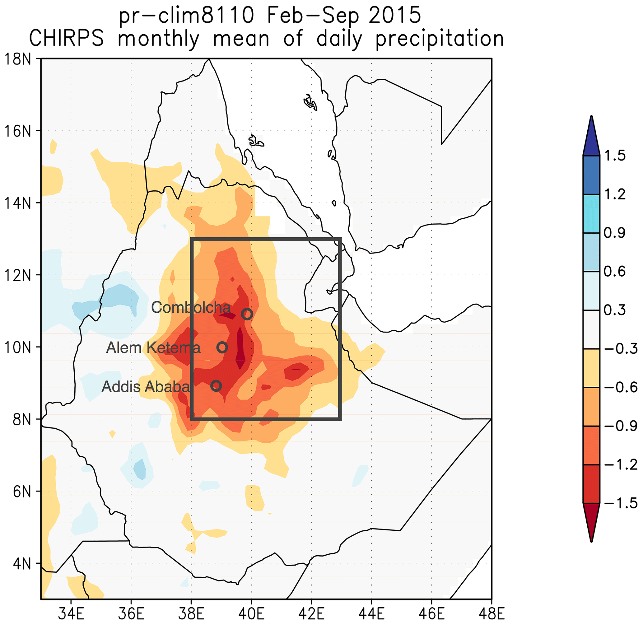
Figure 1 Event definition of the drought event in February–September 2015 in Ethiopia; the box shows the spatial extent of the event definition and the circles show the three station locations. Colours show the anomaly in precipitation (CHIRPS, precipitation minus 1981–2010 climatology) averaged over February–September 2015 (mm d⁻¹). See Philip et al. (2018c) for more details.

For flooding studies ideally hydrological models should be used to attribute water level or maximum run-off at the point where the flooding caused impacts. This has been done for a few slow studies (Schaller et al., 2016; Philip et al., 2019) but is not yet commonplace. In many cases precipitation averaged over the catchment area, or an approximation of it, has been used as a proxy (van Oldenborgh et al., 2012b; Schaller et al., 2014; van der Wiel et al., 2017; van Oldenborgh et al., 2017; Otto et al., 2018a). Philip et al. (2019) showed that for the case of flooding in Bangladesh on the Brahmaputra River, the results for time- and space-averaged precipitation and discharge were comparable (Fig. 2).

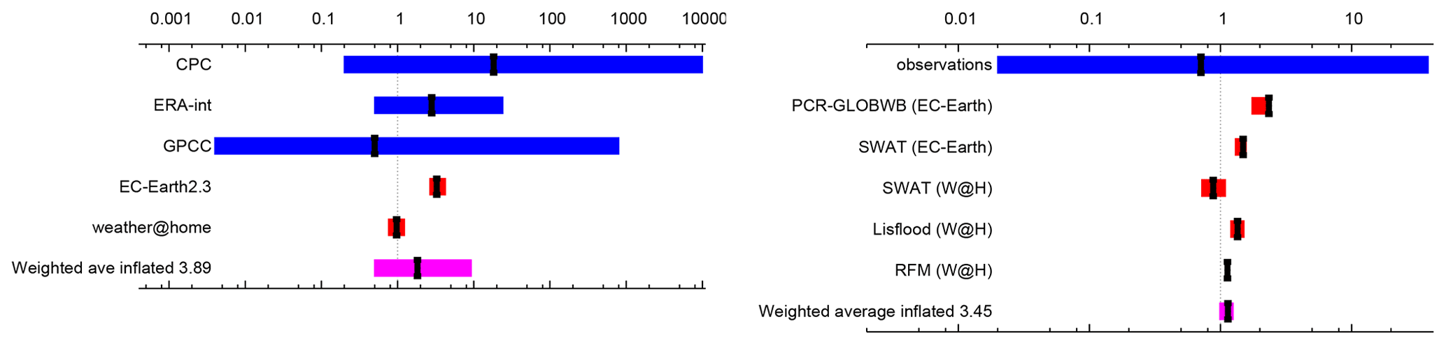
Figure 2 Synthesis of the probability ratios between pre-industrial and 2017 of the precipitation (left) and discharge (right) results. Dark blue is observations, red is climate model ensembles, and the weighted average is shown in purple. The ranges of the models are not compatible with each other, pointing to model uncertainty playing a role over the natural variability. The weighted average has been inflated by factors of 3.89 and 3.45 for precipitation and discharge respectively to account for the model spread. Reproduced from Philip et al. (2019) under the licence agreement at https://creativecommons.org/licenses/by/4.0/ (last access: 31 October 2018); see original paper for more details.

For small-scale precipitation events it is often feasible to pool observations or grid points over a homogeneous region that is larger than the events in order to increase the number of independent events and hence give more precise results. Alternatively, the spatial maximum over this region can be taken; this selects more extreme events than at individual or pooled stations (grid points). A useful homogeneity check is to make a map of the mean of the maximum N-day average of precipitation and require that this does not vary by more than e.g. 20 % over the selected region. This is often the case for flat terrain. Remaining differences can be reduced by scaling each series by this mean before the rest of the analysis. If the maximum is used, the number of stations in the region should be almost constant. The spatial maximum was used as event definition in Vautard et al. (2015), Eden et al. (2016), van der Wiel et al. (2017), van Oldenborgh et al. (2017), Eden et al. (2018), and Luu et al. (2018).

3.4 Choice of timescale

Similarly, the timescale of the event should ideally correspond to the impacts as well, which can differ from location to location due to different vulnerabilities. Limitations on the timescale stemming from knowledge and validation of climate model data (see also Sect. 5) can feed back into this step. If the main effect of heat in India is on outdoor labourers, instantaneous afternoon temperature or heat index would be obvious choices. However, if the literature suggests that longer-duration heat waves have correspondingly more impact, such as in Europe (D'Ippoliti et al., 2010) probably because the vulnerable population there is elderly and indoors, a 3-day average may be more appropriate.

For meteorological droughts, a precipitation deficit over a number of months or years can be taken, which is available from global climate models. However, for agricultural or hydrological droughts, hydrological models must be used to get soil moisture or river discharge data. This is often challenging due to lack of long-term observational data (e.g. Kew et al., 2020; Kam et al., 2018) and a mismatch of the horizontal scale (Kam et al., 2018). For flooding the situation is similar: instantaneous water levels are usually a good measure. If those observations are not available, precipitation averaged over the response time of the basin can be a good substitute (Philip et al., 2019). Sometimes the relevant timescale is too short to be resolved by observations and models, for instance a flash flood event from a thunderstorm lasting 1 h. In that case the nearest useful scale must necessarily be chosen, in this case often daily precipitation.

Finally, the seasonality of the event has to be taken into account. Most often, the impact of an event is independent of the season in which it occurs, so that all seasons can be included in the definition (highest temperature, precipitation, etc., of the year). However, sometimes the impacts vary with the seasons, usually because of missing physical impact modelling. For instance, the 2013 rains in central Europe led to more severe flooding than other more extreme rainfall events in the area because they occurred early in the summer. In this case the rain fell on saturated soils and snow that melted, so that the amount of runoff was much larger than for equal-size precipitation extremes in late summer. Without a hydrological model describing these factors, restricting the analysis to early summer avoided the comparison with late-summer events (Schaller et al., 2014).

The distribution of temperature extremes also varies greatly with the seasonal cycle, so that the analysis has to be restricted to certain months if it is not a heat wave in the summer season or a cold wave in the winter season. If the extremes occur in a season with a strong seasonal cycle, meteorological extremes are best studied as anomalies. However, the impacts are usually dependent on absolute thresholds of temperature.

3.5 Motivation of choices

For an attribution study in response to a high-impact extreme meteorological event, both the spatial and temporal definitions can either be based on the impacts or on the rarity of the meteorological event. The return period of the event can be very sensitive to this choice. A definition that optimizes the location and duration on the meteorological extreme event logically results in very high values for the return period. On the other hand, people can experience large impacts even when the event is not very extreme meteorologically (e.g. Siswanto et al., 2015), and meteorologically extreme events can have relatively small impacts (e.g. Sun et al., 2018; van Oldenborgh et al., 2018). The choice whether to optimize the event definition for meteorological rarity or to describe the impacts should be documented.

At the end of step 2 the event definition should be written down clearly in terms of variable (e.g. maximum daily temperatures, daily precipitation), spatial extent (area average or point location), temporal extent (e.g. 3-day average, seasonal average), and over which season (e.g. summer, rainy season, whole year). Examples are the following.

• The lowest minimum temperature of the year at Chicago Midway station (and De Bilt) (van Oldenborgh et al., 2015),

• the highest 3-day averaged station precipitation along the US Gulf Coast, 29–31^∘ N, 85–95^∘ W (van der Wiel et al., 2017),

• the maximum 3-day averaged precipitation averaged over the Seine (and Loire) basin in April–June (Philip et al., 2018b), and

• the lowest 3-year averaged precipitation around Cape Town, 35–31^∘ S, 18–21^∘ E.

4 Step 3: Observed probability and trend

The third step is trend detection. This is the process of determining whether there is a trend detectable above the natural variability in observational data for the class of events defined in step 2. The return period of the event in the current climate conditions can also be determined from observations at this stage. A trend may not yet have emerged from the noise in the observations even though the probability of the event has changed. So the absence of a significant trend would not lead by itself to a non-attribution statement. It is important to note that detected trends may arise for a different reason than a change in global climate forcing.

4.1 Observational data

The first task is to analyse observational data. The ideal situation is to have 150 years of homogeneous observations up to and including the event under analysis. However, this is hardly ever the case, and one is often left with shorter (or inhomogeneous) series in practice. Given the limited amount of data available, a major consideration is to use them as effectively as possible. Considerations are outlined below.

For observations there are two types of data: local and regional. Local data mainly consist of station data time series. Regional data can be obtained from gridded observations (statistically interpolated station observations) and reanalyses (using a weather model to assimilate all kinds of observations). Satellite-derived products have not yet proven themselves to be useful due to their short records, often with discontinuities, and large biases compared to ground observations. Radar observations of precipitation are more reliable when calibrated against station data but do not extend far enough back in time for trend analysis.

For extremes, station data are in general more reliable than gridded data because gridded data may contain information from varying numbers of stations per grid box rather than a uniform set of stations. This affects the variability of the gridded data time series (Hofstra et al., 2009, 2010). If the distance between stations is larger than the decorrelation scale, the variability in the interpolated grid boxes will be too small (King et al., 2013a). We discuss the two extreme scenarios of numbers of stations per grid box. On the one hand, in the extreme case that no station information is available and values are set to climatology, the analysis will give climatology with no variability. On the other hand, if the number of stations per grid box is large, averaging over these stations will result in averaging of local-scale variability with the effect of reducing overall variability. We recommend always checking the documentation and meta-data of the datasets on information about the number of stations per grid box and making choices accordingly. This information is often available as a separate field.

Station data are often inhomogeneous in time due to site relocations or changes in the observational methods (Fig. 3a), not to mention misplaced decimal points (Fig. 3b). Comprehensive quality control should eliminate the latter. When available, homogenized station data should be used, even though the homogenization is often only in the mean, not the variability. Long time series such as Central England Temperature (Parker et al., 1992; Manley, 1974) (starting in 1659) and the Dutch De Bilt series (starting in 1706) have larger variability before the construction of the modern-day observation networks in the early 20th century (Fig. 3c, d) and hence cannot be used for studying extremes before that. Another insidious problem is trends in missing data: a decrease in missing data gives rise to an increase in the probability of observing extremes and hence a spurious trend (van Oldenborgh et al., 2018). If there is an obvious discontinuity in the mean or variability early on in the dataset, often the dataset can still be used if the years before the discontinuity are omitted.

If the decorrelation length of the extreme under investigation is smaller than the area over which the properties are homogenous, station data can be pooled to give more degrees of freedom than years of data (Buishand, 1991; Katz et al., 2002). This is often the case for convective precipitation events in summer (Vautard et al., 2015; Eden et al., 2016, 2018) but also for 1-day extreme rainfall on the south-eastern coast of India (van Oldenborgh et al., 2016b) and 3-day extreme rainfall events on the US Gulf Coast (van der Wiel et al., 2017; van Oldenborgh et al., 2017). Care has to be taken to take remaining spatial dependencies into account by separating the stations sufficiently and taking moving spatial blocks in the bootstrap procedure (see Sect. 4.2).

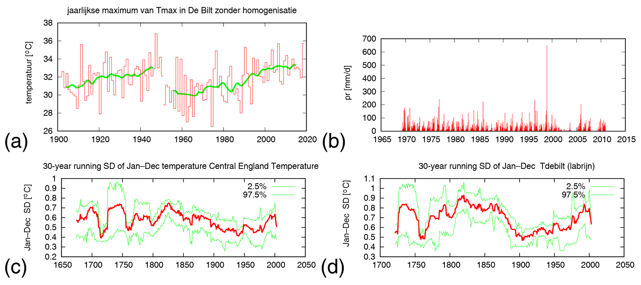
Figure 3 Examples of problems with time series, reproduced on the Climate Explorer at https://climexp.knmi.nl (last access: 31 October 2018). (a) A 2 ^∘C inhomogeneity in the highest maximum temperature of the year, TXx, in 1950–1951 (De Bilt before homogenization; Brandsma, 2016), (b) precipitation at a station illustrating displaced decimal points giving an unrealistic extreme of 660 mm d⁻¹ that does not show up in satellite data, disaster databases or newspapers, and a factor 10 the other way in 2001–2003, (c) 30-year running standard deviation of annual mean Central England Temperature (Manley, 1974; King et al., 2015), and (d) the same for the De Bilt temperature (van Engelen and Nellestijn, 1996).

For a regional average a gridded dataset is usually used. An algorithm weights the station data according to their spatial distribution. As noted above, in many cases, the quality of gridded data varies regionally, either in the historical length of the observational series used as input or in the temporally varying number of stations per grid box. Sharp changes in data quality can occur along country borders, for example. If the gridded dataset is the principal observational data to be used in the analysis, this should be taken into account in the spatial event definition. Sometimes a trade-off between quality and impacts can be made so that the area defining the event is restricted to a region that is more spatially homogeneous in data quality yet is still representative, even if not optimal, for the impacts. For example, Kew et al. (2019) shifted the northern boundary of the long–lat box used for a heat-wave analysis southward to omit a region of poor data homogeneity.

Reanalysis data, which are data from a meteorological model with observational data assimilated into it, incorporate information about many variables rather than only one. In contrast to the statistical interpolation used to grid observational analyses, which would tend to spatially smooth a data field, a meteorological model can generate extremes between point observations (see Hofstra et al., 2009, 2010, for the effect of interpolation on extremes). For this reason, and especially in regions where in situ observations are sparse, we assume that reanalysis data generally contain a more homogeneous representation of extremes in time than gridded observations as long as the extremes are representable by the underlying model, which is e.g. not the case for convective events, so that precipitation in the tropics is not well represented (e.g. Kharin et al., 2005).

The reliability of the data should be at least checked by visual inspection (e.g. Sillmann et al., 2013) and by gathering information on the amount and quality of data used in gridded datasets (observational data and reanalyses). Often information on how the quality of a dataset varies in time or space is given in the dataset's documentation or webpage or can be obtained by contacting the developers directly. Care has to be taken that there is no temporal discontinuity. For example, with the advance of satellite data in the early 1980s, observational-based products that cover some period before and after this date may suffer from a discontinuity or quality differences. If one solely uses data from the 1980s onwards, the statistical uncertainty in trends often becomes large due to the relative short length of the time series. As an alternative, one may consider using long reanalysis products based on a homogeneous subset of data, usually SST and surface pressure observations, disregarding satellite data (e.g. Compo et al., 2011; Laloyaux et al., 2017). These reanalyses that use a subset of the available observational data provide homogeneity over the long time periods required, though at the expense of accuracy in recent decades.

The choice to use local, regional, or both types of data often depends on the availability of a reliable and homogeneous dataset and needs expert judgement. If there are no reliable and homogeneous observational data of the event itself or of the history of similar events, the attribution study cannot be carried out.

4.2 Statistical method

The previous step has provided a long time series up to and including the event. There are many ways to detect changes in the frequency of extreme events in this series. The simplest is to divide the time range into two or more blocks and count threshold exceedances. This has the advantage of making no assumptions about the statistical distributions of the variable in question but has in general a low signal-to-noise ratio; i.e. the uncertainties are large. The statistical uncertainties due to the variability of the weather can be reduced by making assumptions about the shape of the distribution and the kind of changes that are most likely. Within the observational data it can be verified that some of these assumptions cannot be rejected. For others this requires long time series or large ensembles of model data (see Sect. 6).

The main assumptions we make are the following (see also van der Wiel et al., 2017), and these are topics of ongoing research.

• It is assumed the events follow a theoretical distribution, such as a Gamma distribution (based on all data) or one of the extreme value distributions discussed below that is based on events in the tail only. If the event is not very extreme, a normal distribution can also be used. In general this implies that we assume that more moderate extremes behave the same as the more intense extreme that is under investigation, and these provide the higher number of events necessary to detect a trend. A comparison of the observed cumulative distribution function (CDF) to the fitted distribution shows when this assumption does not hold. Depending on the interest field, several distributions can be tested on how well the sample data are fitted by these different distributions by evaluating a quantile–quantile plot or, equivalently, a return time plot that shows the same information but emphasizes the tail. Gaussian distributions are often seen not to describe the tails well. A choice is made based on the comparison.

• It is assumed that the main changes in the distribution are due to global warming. In the global mean temperature, the influence of natural forcings over the last 70 or 120 years has been very small compared to the anthropogenic forcings (Bindoff et al., 2013). If we take the smoothed global mean temperature as a covariate, both anthropogenic and natural forcings are included. Note that while using smoothed global mean temperature we cannot attribute changes to local forcings, such as aerosols, irrigation, and roughness changes, which can also have large influences on extremes (Wild, 2009; Puma and Cook, 2010; Vautard et al., 2010). This should always be kept in mind and checked when possible. If factors other than global warming are important for changes in the distribution, attribution to global warming alone is not appropriate and additional investigation should be conducted. See for instance the analyses of heat in India, in which air pollution and irrigation are as important (van Oldenborgh et al., 2018), and of winter storms in Europe, where roughness appears to be much more important than climate change (Vautard et al., 2019), but also land surface changes in heat extremes in the central US (Cowan et al., 2020).

• It is assumed that the distribution of temperature extremes shifts due to global warming without changing the shape (σ,ξ constant), and for precipitation and wind extremes the distribution scales ($\mathit{\sigma }/\mathit{\mu },\mathit{\xi }$ constant), which keeps the distribution positive-definite. In the latter case an exponential dependence on temperature is inspired by the Clausius–Clapeyron relation. The winds in the more extreme smaller-scale wind storms such as tropical cyclones are to a large extent driven by the energy release. For midlatitude wind storms, which usually show small trends (Vautard et al., 2019), this is a preliminary first-order approximation that ensures that the PDF stays positive-definite, in contrast to the linear shift that is sometimes used. At the moment these assumptions can only be tested using large amounts of model data and only if the data show a forced trend.

• The fits assume all years are independent. In some parts of the world decadal variability is stronger than the variability on the weather scales integrated to decadal variability (which decreased with the square root of the ratio of the weather timescale and the decadal timescale van Oldenborgh et al., 2012a), and this should be taken into account there.

• It is assumed that if the decorrelation length of the extreme is smaller than the region in which they occur with the same properties, the events can be pooled spatially to increase their numbers, taking spatial dependencies into account in the uncertainty estimates. Alternatively, the spatial maximum can focus the fits further towards the extreme tail of the distribution (Eden et al., 2016; van der Wiel et al., 2017; van Oldenborgh et al., 2017).

The result of the fit to a statistical model provides an estimate of the return period of the event of interest and whether there is a trend outside the range of deviations expected by natural variability. Different classes of events require different types of statistical functions. In the next subsections some possible distributions are explained that can be used for different types of events (e.g. Coles, 2001; Katz et al., 2002). Confidence intervals (CIs) have to be estimated: a straightforward method is to use a non-parametric bootstrap, i.e. repeating the fit a large number of times (1000 or so) with samples of (covariate, observation) pairs drawn from the original series with replacement. If there is no a priori evidence of which sign the influence of anthropogenic climate change has on the extreme, a two-sided 95 % CI is appropriate, from 2.5 % to 97.5 % of the bootstrap sample. However, often we know the sign from previous research, e.g. in most regions warming for temperature extremes and intensification of short precipitation extremes when there is enough moisture availability in the absence of overriding dynamical changes. In those cases it may be appropriate to use a one-sided CI, from 5 % of the bootstrap sample.

A thorny question is whether the observed extreme event that triggered the analysis should be used in the fit. It has been observed and hence adds to our knowledge of the distribution of extremes. However, including it also biases the trend towards the extreme as the analysis would not have been done without it: a very hot extreme will give a higher trend. In previous analyses we have chosen not to include the event and answer the question whether we could have known before the event took place whether the probability of this event occurring has changed. We do use the information that it occurred by demanding that the distribution has a non-zero probability of the observed event occurring, also for all bootstrap samples. This primarily affects the uncertainty estimates of temperature extremes, which usually have upper bounds.

4.2.1 Gaussian

Ordinary least-square trend fitting assumes the data are normally distributed. This distribution is also called a Gaussian distribution. Following the central limit theorem, this often describes aggregate quantities such as large-area seasonal means well and has the advantage of having only two parameters to fit plus the trend. However, the tails of the normal distribution decrease as exp (−z²), which is usually more quickly than reality. This implies that this distribution can only be used for moderate extremes with low-return periods that are not in this tail. If a comparison of the empirical CDF with the fitted one indicates that the tails above the event are not fitted well by the Gaussian, a more realistic description of the extremes is needed.

4.2.2 GPD

The generalized Pareto distribution (GPD) is used for extremes above or below a threshold; this method is also referred to as peak over threshold (POT). The GPD gives a three-parameter description of the tail of the distribution. A low tail is first converted to a high tail by multiplying the variable by −1. The high tail of the observed distributions is then fitted with

$$\begin{array}{}\text{(1)}& H(\mathit{\mu }-x)=\mathrm{1}-{\left(\mathrm{1}-{\displaystyle \frac{\mathit{\xi }x}{\mathit{\sigma }}}\right)}^{(-\mathrm{1}/\mathit{\xi })},\end{array}$$

with x the temperature or precipitation, μ the threshold, σ the scale parameter, and ξ the shape parameter determining the tail behaviour. The shape parameter ξ is considered to be unphysical if it is very large (a larger-scale parameter gives a fatter tail). During the fitting procedure, unphysically large shape parameters have to be suppressed, e.g. by a penalty term that keeps them roughly in the range $\left|\mathit{\xi }\right|\le \mathrm{0.4}$ (Katz et al., 2002). For the low extremes of precipitation, the fit is constrained to have zero probability below zero precipitation ($\mathit{\xi }<\mathrm{0},\mathit{\sigma }<\mathit{\mu }\mathit{\xi }$). As mentioned above, for negative shape parameter ξ we also demand that the observed event is below the upper limit.

The POT method can be used for all timescales, but it has mostly been employed for long timescales, e.g. a monthly mean high temperature or a seasonal mean drought (low precipitation values), if a fit to all data with a Gaussian or Gamma function is not appropriate. To apply the POT method to daily data, the threshold exceedances have to be declustered into distinct events, which is not easy to do automatically, so we prefer to compute block maxima and fit to a GEV function.

The choice of threshold in the POT method depends on the trade-off between setting it high to be closer to the limit in which the GPD applies and low to have enough events above the threshold to do a sensible fit. For annual values this implies fitting to the highest 20 % or 10 % of the distribution. This is not very extreme, so the justification from extreme value theory is not very strong. However, it can be seen as a good empirical choice, i.e. a function with enough flexibility to be able to describe the data even if its use cannot be justified on theoretical grounds. Whether the function describes the empirical distribution well can be seen in a quantile–quantile plot or equivalently the return time plot that contains the same information but stresses the extremes. An objective statistical goodness-of-fit test is recommended in addition to the visual inspection of the plots. We try to explore different thresholds to the extent the data allow as recommended by Coles (2001). If the results are not stable, they are not used. An example is the description of low seasonal precipitation extremes for which a Gaussian distribution would give positive probabilities for negative precipitation. In the GPD fit we avoid this by demanding a lower bound that is zero or higher.

4.2.3 GEV

The generalized extreme value (GEV) distribution describes the largest observation from a large sample (block maxima, Coles, 2001). It is thus used for event definitions like the annual maximum temperature or maximum daily precipitation in a season. The GEV distribution can be formulated as

$$\begin{array}{}\text{(2)}& P\left(x\right)=\exp \left[-{\left(\mathrm{1}+\mathit{\xi }{\displaystyle \frac{x-\mathit{\mu }}{\mathit{\sigma }}}\right)}^{-\mathrm{1}/\mathit{\xi }}\right],\end{array}$$

with x the variable of interest, e.g. temperature or precipitation. Here, μ is referred to as the location parameter, σ as the scale parameter, and ξ as the shape parameter determining the tail behaviour. Similar to the GPD distribution, unphysically large shape parameters have to be suppressed, e.g. by a penalty term that keeps them roughly in the range $\left|\mathit{\xi }\right|\le \mathrm{0.4}$.

An extension is to use an agreed number of the r largest values per year (Coles, 2001). This gives more data points and hence smaller uncertainties due to natural variability but requires declustering and implies estimating the behaviour of the extreme from more moderate extreme events.

4.2.4 Gumbel

In cases where the shape parameter ξ of a GEV distribution becomes zero, the distribution is referred to as a Gumbel distribution. This can sometimes also be achieved by transforming the variable of interest. For instance, in many regions, daily precipitation can be transformed to a Gumbel distribution by raising the precipitation to the power 3∕2 (van den Brink and Können, 2011). As for the Gaussian distribution, the Gumbel distribution results in a smaller uncertainty range and can be used when a Gumbel model fits the data sufficiently well and there are physical arguments as to why the shape parameter should be zero.

4.2.5 Gamma

The gamma distribution is often used to describe the distribution of precipitation. For daily precipitation it is augmented with a fraction without measurable precipitation (P<1 mm usually). It has been used with a covariate in for instance Gudmundsson and Seneviratne (2016).

$$\begin{array}{}\text{(3)}& G\left(x\right)={\displaystyle \frac{\mathrm{1}}{\mathit{\sigma }\mathrm{\Gamma }\left(\mathit{\xi }\right)}}(x/\mathit{\sigma }{)}^{\mathit{\xi }-\mathrm{1}}\exp (-x/\mathit{\sigma }),\end{array}$$

with σ the scale parameter and ξ the shape parameter. For daily data or data sampled of the order of a few hours to a few weeks, a fraction of wet days n is included:

$$\begin{array}{}\text{(4)}& G\left(x\right)=(\mathrm{1}-n)\mathit{\delta }\left(x\right)+{\displaystyle \frac{n}{\mathit{\sigma }\mathrm{\Gamma }\left(\mathit{\xi }\right)}}(x/\mathit{\sigma }{)}^{\mathit{\xi }-\mathrm{1}}\exp (-x/\mathit{\sigma }),\end{array}$$

with δ(x) the Dirac delta function, a peak with width zero and integral one.

4.3 Trend definition

To calculate a trend in transient data, some parameters in these statistical models are made a function of an indicator of global warming (or another covariate; the same methods can be used to investigate the dependence on e.g. El Niño–Southern Oscillation, ENSO). For global warming a common choice is the 4-year smoothed global mean surface temperature (GMST) anomaly, T^′, the “pattern scaling” technique (Tebaldi and Arblaster, 2014). The smoothing is introduced to remove the fluctuations in the global mean temperature due to ENSO, which would contaminate the global warming fingerprint with ENSO teleconnections. Taking other measures, such as the atmospheric CO₂ concentration or radiative forcing estimates, gives almost the same results as these are highly correlated: for annual means, the Pearson correlation coefficient between CO₂ concentration and smoothed GMST is $r(T^{\prime },{\mathrm{CO}}_{\mathrm{2}})=\mathrm{0.93}$. However, a linear trend in time misses the non-linear increase in radiative forcing and the resulting warming trend and hence in principle does not fit the data as well. Linear trends in time also depend more strongly on the starting date. The same holds for non-parametric trend tests such as the Mann–Kendall test, which does not take into account the time evolution of the climate change signal.

The covariate-dependent function can be inverted and the distribution evaluated for a given year, e.g. a year in the past (with $T^{\prime }=T_{\mathrm{0}}^{\prime }$) or the current year ($T^{\prime }=T_{\mathrm{1}}^{\prime }$). This gives the probabilities for an event at least as extreme as the observed one in these 2 years, p₀ and p₁, or expressed as return periods ${\mathit{\tau }}_{\mathrm{0}}=\mathrm{1}/p_{\mathrm{0}}$ and ${\mathit{\tau }}_{\mathrm{1}}=\mathrm{1}/p_{\mathrm{1}}$. We estimate confidence intervals using a non-parametric bootstrap procedure. If the one- or two-sided confidence interval on the PR excludes one (no change), the distribution is significantly different between the two climates.

4.3.1 Shift fit

In the case of a temperature event, it is commonly assumed that the trend shifts with GMST. This assumption has been found to hold well in some studies using large ensembles of model simulations with enough data to analyse them without relying on statistical fits (Sippel et al., 2016; Kew et al., 2019). For observational studies this assumption implies fitting the temperature data to a distribution that shifts proportionally to the smoothed global mean temperature: $\mathit{\mu }={\mathit{\mu }}_{\mathrm{0}}+\mathit{\alpha }{T}^{\prime }$ and σ=σ₀, with α the trend that is fitted together with μ₀ and σ₀. The shape parameter ξ is assumed constant. The change in magnitude of the extreme events is independent of the magnitude of the event (by assumption) and equal to $\mathrm{\Delta }I=\mathit{\alpha }(T_{\mathrm{1}}^{\prime }-T_{\mathrm{0}}^{\prime })$. The change in probability (PR) does change with the magnitude, for heat events often vary strongly. If the one- or two-sided 95 % confidence interval excludes zero, the change is statistically significant.

Otto et al. (2018b) for instance analysed the cold wave in June–August 2013 in Peru assuming that the trend in minimum temperatures shifts with smoothed GMST. They did this by investigating the CRU TS4.00 minimum temperature time series. Whilst both Gaussian and GPD distributions fit the data well, minimum temperatures over June–August were fit with a normal distribution that shifts with the global mean surface temperature. The return period of the 2013 cold event was calculated to be 17 years (95 % CI 7 to 75 years); see Fig. 4. In the past, such cold events happened more often: the probability ratio is 0.08 (95 % CI 0.02 to 0.21); i.e. these events occurred 4 to 50 times more often before the bulk of anthropogenic global warming took place. As neither event was very unlikely, the use of the normal distribution is justified.

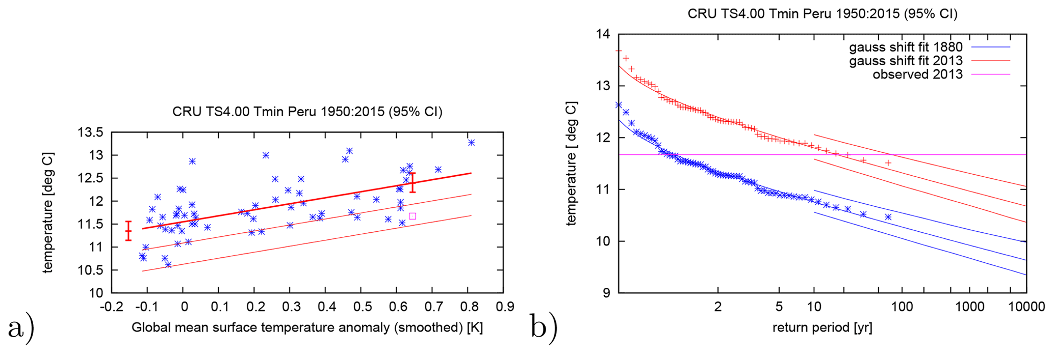
Figure 4 Fit of the minimum temperatures averaged over June–August and Peru. A normal distribution is used that shifts with the global mean surface temperature. The distribution is evaluated for the climates of 1880 and 2013. (a) June–August minimum temperatures against the change in GMST. The thick line denotes the time-varying mean and the thin lines are 1σ and 2σ below, respectively. The purple square shows the 2013 value, which was not used in the fit, and the two vertical red lines show the 95 % confidence interval of μ for the climates of 1880 and 2013. (b) Return periods for the 2013 climate (red lines) and the 1880 climate (blue lines with 95 % CI). Observations are shown twice, once shifted up to the climate of 2013 with the fitted trend (red signs), once shifted down to 1880 (blue signs). After Otto et al. (2018b), reproduced on the Climate Explorer at https://climexp.knmi.nl (last access: 2 December 2019).

An example of a high temperature extreme is the high temperature in De Bilt in 2018 shown in Fig. 5 (van Oldenborgh, 2018). The record for the highest daily mean temperature was broken by 1.6 ^∘C. A fit of the homogenized observations since 1901 gives a trend of 2 to 4 times the global mean temperature and a return period in the current climate of very roughly 300 years (95 % CI of more than 30 years). The observed value is far above the upper limit of the GEV for the year 1900, so formally the event was impossible in the climate of 1900 and the PR is infinite. However, this depends on a number of assumptions, so we prefer to say that the event was extremely unlikely around 1900.

Figure 5 Fit of a GEV of the highest daily mean temperature of the year at De Bilt, the Netherlands, for 1901–2017, shifting with the smoothed GMST, with the value for 2018 (29.7 ^∘C) in purple. (a) As a function of GMST, the thick lines denote μ, the thin lines the 6- and 40-year return periods. (b) As a function of return period in the climate of 1900 (blue) and 2018 (red). After van Oldenborgh (2018).

4.3.2 Scale fit

For precipitation time series or variables related to (lack of) precipitation or wind it is assumed that the distribution scales with GMST. To allow for a trend in probability the threshold or position and scale parameters are dependent on the smoothed global mean temperature T^′ with a trend α such that their ratio is constant. Assuming that the ratio σ∕μ, also called the dispersion parameter, is constant reduces the number of fit parameters. This is a standard method in hydrodynamics, where it is part of the index flood assumption (e.g. Hanel et al., 2009). This assumption has been tested and justified in some studies using large ensembles of model simulations giving large-sample statistics that do not need assumptions about the fit (e.g. Otto et al., 2018a; Philip et al., 2018b). The scaling is taken to be an exponential function of the smoothed global mean temperature, similar to the dependence of the maximum moisture content in the Clausius–Clapeyron relations. This exponential dependence can clearly be seen in the scaling with daily temperature in regions with enough moisture availability (Allen and Ingram, 2002; Lenderink and van Meijgaard, 2008). The whole distribution is thus scaled with

$$\mathit{\mu }={\mathit{\mu }}_{\mathrm{0}}\exp (\mathit{\alpha }{T}^{\prime }/{\mathit{\mu }}_{\mathrm{0}}),\mathit{\sigma }={\mathit{\sigma }}_{\mathrm{0}}\exp (\mathit{\alpha }{T}^{\prime }/{\mathit{\mu }}_{\mathrm{0}}),$$

with fit parameters ${\mathit{\mu }}_{\mathrm{0}},{\mathit{\sigma }}_{\mathrm{0}},\mathit{\alpha }$ and ξ. The shape parameter ξ is assumed constant. Similar to the fits with a shift with GMST, the precipitation distribution can be evaluated for different covariates $T_{\mathrm{0}}^{\prime }$ and $T_{\mathrm{1}}^{\prime }$ giving rise to a probability ratio PR. The relative change in magnitude is now assumed to be independent of magnitude, so it is expressed as a percentage change between the two climates, $\mathrm{100}\mathrm{\Delta }I/I=\mathrm{100}\left[\exp \right(\mathit{\alpha }(T_{\mathrm{1}}^{\prime }-T_{\mathrm{0}}^{\prime })/{\mathit{\mu }}_{\mathrm{0}})-\mathrm{1}]$.

Van der Wiel et al. (2017) studied the August 2016 flood-inducing extreme precipitation in southern Louisiana by looking at 3-day averaged precipitation values. For this they used the 19 stations with at least 80 years of data and at least 0.5^∘ of spatial separation between stations on the central US Gulf Coast. Using a GEV that scales with GMST, they found a return period of about 500 years (95 % CI 360 to 1400) and an increase in probability of a factor of 2.8 (95 % CI 1.7 to 3.8), corresponding to an increase in intensity of 17 % (95 % CI 10 to 21 %) (see Fig. 6). The stations are not all independent, so the bootstrap includes blocks of all stations with cross-correlations $r>\mathrm{1}/e$, on average 2.3 stations, leaving about eight degrees of freedom.

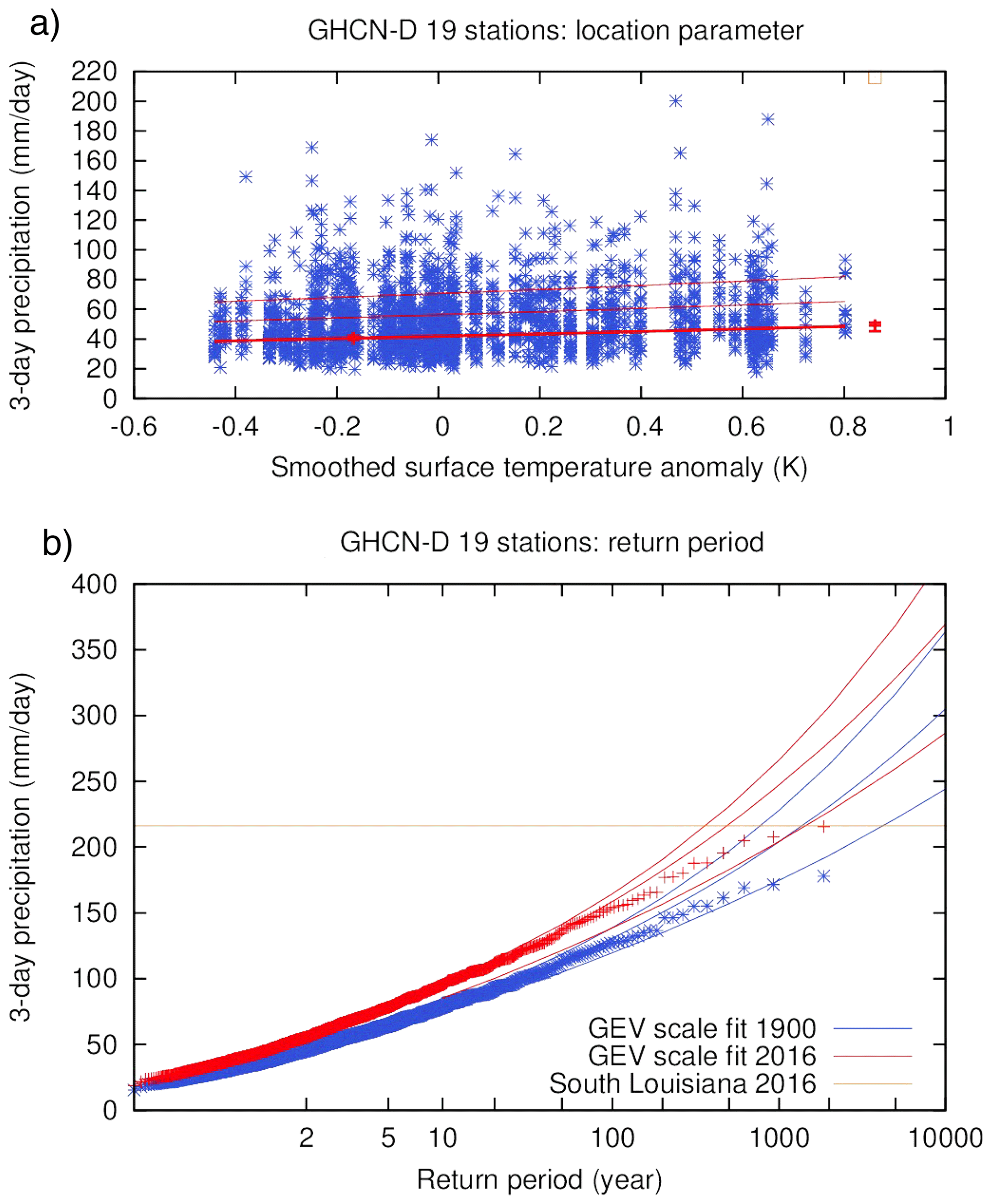
Figure 6 Similar to Fig. 5 but for the extreme precipitation event in southern Louisiana in August 2016, using a GEV distribution that scales with GMST and evaluated for the years 1900 and 2016. Reproduced from van der Wiel et al. (2017) under the licence agreement at https://creativecommons.org/licenses/by/4.0/ (last access: 31 October 2018); see original paper for more details.

4.3.3 Shift and scale fit

The other part of the index flood assumption, that the PDF scales, i.e. σ∕μ is constant, can also be relaxed so that two trend parameters need to be estimated from the data. This has been attempted by Risser and Wehner (2017) but of course results in larger quantified uncertainties.

4.4 Influence of modes of natural variability

It is well known that ENSO has a major influence on temperature and precipitation variability in large parts of the world. The influence is not significant everywhere or in every season: there are for instance very weak ENSO teleconnections in Europe. The link between the magnitude of ENSO, expressed as the monthly relative NINO3.4 index, and the mean temperature or precipitation data in the study area can be analysed to quantify the influence of ENSO by calculating a (lagged) correlation. For instance, Philip et al. (2018c) calculated the difference in return period between the actual drought in 2015 in Ethiopia, with El Niño conditions, and the same drought if it had occurred under ENSO-neutral conditions (detrended NINO3.4 values close to zero). The influence of ENSO, given by the regression slope of the NINO3.4 index on the log precipitation series, was subtracted from 2015 only and the changes to the event's magnitude and return period under ENSO-neutral conditions were investigated, with the rest of the time series unchanged. The actual return period was once every few hundred years (lowest estimate of 60 years, according to the 95 % CI), but under ENSO-neutral conditions the fictitious event would have had a return period of 80 years (lowest estimate of 20 years, according to the 95 % CI). This means that the drought would have been less severe but still exceptional without the influence of El Niño.

Decadal variability can often mask the presence of a background trend due to global warming, particularly when an observational series is too short, which would render an event unsuitable for further analysis. Fortunately, in some cases, decadal variability in the observed time series can be characterized by a known index of a mode of variability. If the correlation between the time series and the index is large and there is a known physical reason for it to be, the index is considered to describe the decadal variability well, and it can be used to remove the decadal signal from the time series. If, after removal of the decadal signal, there is no longer any autocorrelation, only high-frequency variability remains and the observational series can be used for trend detection. For example, van Oldenborgh et al. (2016a) found that the decadal variability in winter temperatures over the North Pole region was highly correlated with the Atlantic Multidecadal Oscillation (AMO) index of van Oldenborgh et al. (2009), which is independent of the warming trend and emphasizes the northern part. Using the regression of the observed series on the AMO to linearly subtract the influence of the decadal variability from polar temperatures left only high-frequency variability, and the resulting time series of temperatures reduced to AMO-neutral showed a significant linear trend with respect to GMST. As the event year was AMO-neutral, the AMO did not change the magnitude of the event in 2016.

Murakami et al. (2015) found that the favourable condition of El Niño and decadal variability interplayed with anthropogenic forcing such that the observed trend in tropical cyclones over Hawaii was not statistically significant, while anthropogenic forcing contributed to the active tropical cyclone season in 2014.

5 Step 4: Model evaluation

From step three, a return period and an observed trend are obtained, as change in probability (PR) and intensity (ΔI). The next step is to attribute these trends to anthropogenic climate change (or other factors, as specified in Sect. 3). This can only be done with physical climate models that solve the physics of the climate system numerically dependent on the external forcing prescribed. These usually also have the advantage of a larger number of data points, as they can simulate the climate many times over. This leads to smaller confidence intervals due to natural variability. However, this comes at the expense of systematic deviations from reality due to model biases. Before they are used one must ascertain that the models are fit for purpose, i.e. that they can represent the particular extreme under study well enough.

It is important to start the model evaluation with as large a set of different climate models as possible. The first reason for this is pragmatic: climate models have in general not been designed to represent extreme events well, and in practice many models have been found not to be fit for this purpose. Starting with a large set of models increases the probability that there are a few that pass the tests described in this section.

This second reason is that single models usually do not give a reliable description of the probability distribution of trends in the climate system: they underestimate the uncertainty (Annan and Hargreaves, 2010; Yokohata et al., 2012; van Oldenborgh et al., 2013), even for perturbed parameter ensembles. The same holds for seasonal forecasts (Hagedorn et al., 2005). Different models all have their specific advantages and disadvantages due to the specific model set-up, e.g. a coupled model, an atmosphere-only model, a very large ensemble or a set of coupled global climate models, transient model runs, or fixed forcing runs. However, there is also a trade-off between the wish to have the results relatively quickly and the availability of model runs. In a rapid extreme event attribution study, the quick availability of model runs also plays a role in the consideration of models that are appropriate to use for the analysis. The use of different models allows a determination of a model spread as an indication of model uncertainties and can give, if the model analyses agree, greater confidence in the results.

The validation consists of three steps:

1. general properties,

2. statistical description of extremes, and

3. physical causes of extremes.

The first step starts with the obvious question of whether the model's resolution and other properties allow it to represent the extreme under study. A model with a resolution of 200 km simply cannot represent a tropical cyclone with features of 25 km or convective events of a few kilometres. To represent a tropical cyclone somewhat realistically, one needs 25 km resolution (Murakami et al., 2015); for short-duration precipitation extremes one typically needs to use a non-hydrostatic model with about 1 km resolution (Kendon et al., 2014). Similar checks should be done for orography when relevant. It is also good practice to compare the seasonal cycle and the spatial pattern of the variable to observations, especially if there are geographical features like mountains or coastlines.

For the statistical comparison of extremes we check whether the fit parameters of the distribution agree within uncertainties with those of the observations determined in the previous step. We allow for an overall bias correction, additive for temperature and multiplicative for precipitation and wind.

In the assessments, if the confidence interval of the remaining fit parameters σ (temperature) or σ∕μ (precipitation, wind) and of ξ (if appropriate) overlap with the intervals of the parameters fitted to observations, the model is considered to be good enough. The trend parameter α can also be compared to the observed value, but this can only be used as a check if the source of the discrepancy is known and prevents a realistic simulation. An example is the trend in the warmest afternoon of the year over India in CMIP5 models, which show a strong warming trend. The observations show no trend due to increasing aerosol concentrations and increasing irrigation (van Oldenborgh et al., 2018). The irrigation is not included in CMIP5 models and the aerosol influence is likely underestimated, so in that case it was decided that these models are not good enough for studying trends in heat waves in India. Note that in all cases the uncertainty due to natural variability can hide systematic deficiencies of the model.

The interplay between biases and natural variability was illustrated by Kew et al. (2019), who studied the European heat wave of summer 2017 in 3-day averaged maximum temperatures. In that particular study, model validation revealed that the models that were available overestimated the variability of high extremes of temperature averaged over a large area in the Balkans. Therefore a formal attribution to anthropogenic climate change was not possible for this area. Some models could however be used to study station locations, partly because the uncertainty in the fit parameters is larger for individual stations than for an area average, so that the test is less powerful for individual stations.

The third step is evaluation of the physical characteristics of the extremes: does the model generate these extremes for the right reasons? This is still a subject for research (Vautard et al., 2018) and we only have a few partial answers on how to investigate this at this moment. Useful checks have been whether the ENSO teleconnections to the extreme are realistic (King et al., 2016) and whether the modelled meteorological conditions that cause extreme precipitation on the US Gulf Coast look realistic and include one-third of non-hurricane events (van der Wiel et al., 2017). Tracing back the source of water of an extreme precipitation event turned out to be less useful as the sources can differ widely between different events in the same area (Eden et al., 2018). Apart from the evaluation of the physical cause of extremes, the response of extremes to external forcing should be evaluated. We expand on this in Sect. 7 on hazard synthesis.

A by-product of the statistical check is that it provides information on any model biases. A bias correction usually needs to be applied before the model can be compared to the observations. The most straightforward way is to apply a bias correction to the full distribution. An additive bias correction would be given by the differences in μ between the model and observations and a multiplicative one on μ∕σ. This method (or, alternatively, adjusting the extreme value) was used in earlier analyses when μ of the model was outside observational uncertainty bounds and no anomaly series was used. However, this method often gives rise to return values in the model that are very different from the observed ones. A simpler method is to just evaluate the model for the same return period as we found in the observations. This implies that we keep p₀ fixed and give up the possibility of estimating the return period from models.

In some cases an ensemble consists of different models pooled together, e.g. the EURO-CORDEX regional climate simulations. In that case all models have to be bias-corrected individually. Alternatively, a version that has already been bias-corrected can be used (see e.g. Kew et al., 2019; Vautard et al., 2019; Luu et al., 2018), However, these bias corrections were not designed specifically for the extremes and a specific assessment is still necessary in this case. Luu et al. (2018) proposed a testing procedure for this. In such studies pre-bias-corrected sets were compared with simple scaling corrections, and results were found to be similar.

Philip et al. (2019) analysed the August 2017 floods in Bangladesh from meteorological and hydrological perspectives. In the meteorological analysis they fitted the 10-day averaged precipitation over the Brahmaputra basin to a GEV that scales with GMST. The event amplitude was found to be 14.2 mm d⁻¹ using the CPC dataset, and the associated return period was found to be 11 years (though with a large uncertainty). In one of the models they used (EC-Earth), which passed the validation tests for the GEV fit for the same period as used for CPC and with scaling to GMST, the return period of 11 years corresponds to 16.9 mm d⁻¹ averaged over 10 days. For the calculation of the probability ratio in that model a threshold value of 16.9 mm d⁻¹ was therefore used.

Recently a few issues on reliability and calibration have been raised in the literature. In the next few paragraphs we describe implications specifically for the attribution studies and methods addressed in the present paper.

There have been arguments that we should also assess and correct the reliability of the ensembles (Bellprat and Doblas-Reyes, 2016; Bellprat et al., 2019), although others found that the reliability of attribution statements is only weakly connected to the reliability of the ensemble (the term used in forecast verification) (Lott and Stott, 2016; Ciavarella et al., 2018). This depends crucially on the framing of the attribution question. For the simple framing we use here, with only the trend describing deviations from the climatology of the ensemble, the requirement that the fit parameters (trend, scale, and shape parameter) of the model ensemble agree with the fit parameters of the observations already ensures that the reliability is good, as the natural variability is totally uncorrelated between the observations and models. In case the rapid attribution would be carried out with actual or forecast SSTs (which is currently not the case), correlating the study variable with SSTs on a global map should reveal whether there is a teleconnection in the observations, assuming this type of teleconnection is most important for our rapid attribution studies. In a global map these teleconnections appear as correlations of SST with the variable in the area under study. However, if there is no teleconnection in the observations but a spurious one in a model, as in the example of Bellprat et al. (2019), a reliability test may be useful.

Bellprat et al. (2019) also propose a calibration procedure to correct an unreliable ensemble by adjusting the trend and variability to the observed values. The calibration constants are however of the same order of magnitude as the uncertainties in the trend and variability of the observations, which is usually much larger than for models. Currently, their technique does not propagate the uncertainties in these calibration constants. Not including these uncertainties would give rise to a severe underestimation of the uncertainty of the attribution statement, so they would need to be taken into account if this calibration procedure would be used.

More fundamentally, this procedure would result in reproducing the trend from gridded observations. As we use the models to investigate whether we can attribute the observed trend to climate change or not, it is important that the factors influencing the model trend are independent of observations. Effectively setting the model trend equal to the observed one would negate that use of the climate models. If there is a discrepancy between observed and modelled trends, this can point to the existence of additional trend-influencing factors in the real world that are not adequately represented in the climate models. This gives rise to a very different attribution statement than one would obtain after setting the modelled trend equal to the observed one. If models fail to pass the validation criteria we use, rather than applying a calibration procedure to align the output to observations, we recommend that the (physical) processes in those models leading to differences with observations are first investigated.

The result of this fourth step, the model evaluation, is a list of models that can be used for further analysis of the extreme event, including information on the validation and threshold values. In the case that fewer than two models pass the validation test, we do not accept it as a robust attribution statement anymore, as a single model is usually overconfident.

6 Step 5: Multi-method multi-model attribution

The fifth step in the attribution study comprises the actual attribution analysis. After defining the threshold value the trend and probability ratio can be calculated from the model distributions. In previous studies two types of model ensembles have been used that require different approaches. These are “fixed forcing” runs and “transient forcing” runs.

6.1 Fixed forcing runs

The original proposal for event attribution (Allen, 2003) was for two model experiments, one for current conditions and one for a counterfactual world without anthropogenic emissions and hence pre-industrial concentrations of CO₂ and other greenhouse gases as well as aerosols. Note that current conditions are conditions we experience in the current transient climate and not in a possible future equilibrium state. SST-forced models obviously need adjusted SSTs and sea ice, usually from coupled experiments. It is preferable to sample the uncertainty in the amplitude and pattern by using a set of different pre-industrial SST fields (Schaller et al., 2016). Some models also adjust the land surface between these climates, others keep it the same.

The calculation of the probability ratio requires separate calculations for the probability from the counterfactual forcing experiments and the current forcing experiments. This is determined either by non-parametric methods (counting) or fits to extreme value functions (better precision but more assumptions; see Sect. 4.2 for statistical models used). The threshold value is again obtained by means of setting the return period in the current conditions' run equal to the value from observational data. The probability ratio is simply the ratio of the two probabilities (or return periods). A confidence interval is easily estimated from the CIs of the two probabilities, as these are independent. The same procedure can be used for the estimation of change in intensity of the event, ΔI.

Otto et al. (2018a) studied the flooding event in northern England and Scotland of December 2015 that was caused by heavy precipitation during storm Desmond. The weather@home ensemble was used to simulate the current climate (“actual” ensemble) and a counterfactual climate without anthropogenic climate change but the same SST anomalies (“counterfactual” ensemble). For this very large ensemble no assumption was needed about the distribution. The return period of a 1-in-5-year event in the current climate would have been an approximately a 1-in-10 (95 % CI 6 to 18) year event in the counterfactual “world that might have been” without anthropogenic climate change. This gives an increase in the likelihood of such an event occurring of a factor of 1.3 to 3.5 (see Fig. 7).

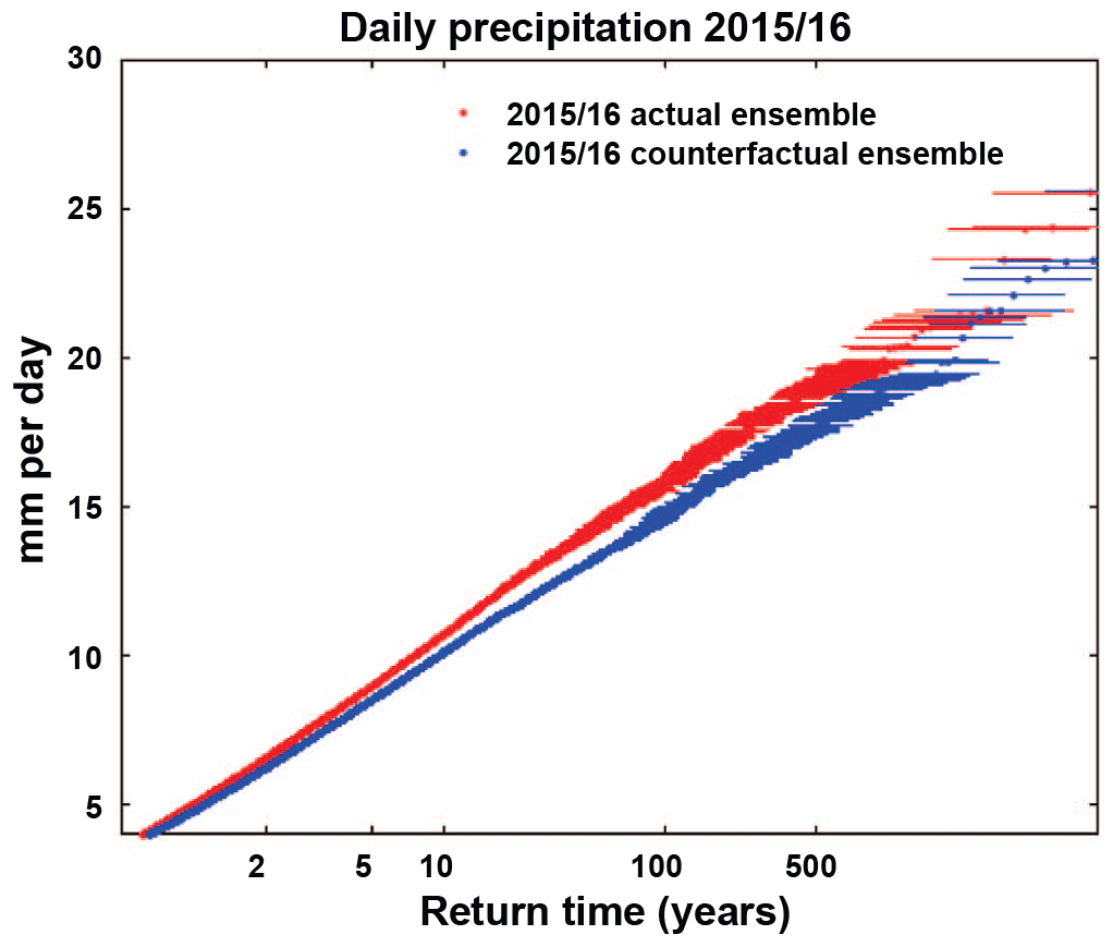
Figure 7 Probability plot for the maximum of winter (DJF) daily precipitation averaged over the northern UK, 54–57^∘ N, 6^∘ W–2^∘ E. Red indicates the probability of daily mean precipitation under observed climate conditions, blue the counterfactual simulations without anthropogenic climate change. See Otto et al. (2018a) for more details.

If the model is run under a future scenario forcing, the same method can be used to analyse the future scenario, for instance for a 2 ^∘C warmer world. With this, a statement on the future probability of the event under consideration can be made for this model.

6.2 Transient forcing runs

An alternative is to use transient forcing experiments and analyse them in the same way as the observational data, except that multiple ensemble members may be available. If the attribution is done conditional on some mode of variability, e.g. ENSO, members in the prescribed phase can be selected (King et al., 2013b). The selected ensemble members are included in the same fit, and years from the past until current conditions are used in this analysis. (Current conditions can be the current year but also the model year in which modelled global mean temperature has risen the same amount as the observed one.) It is preferable not to include data up to the end of the integrations, often 2100. This would increase the signal-to-noise ratio, but local forcings often have very different influences in the future than in the past. For instance, aerosol effects tend to increase up to now and may decrease in the future depending on the scenario definition.

Using the threshold value for which the return period in the model is similar to that of the observed extreme event, the trend and probability ratio can be calculated for the years Y₀ and Y₁. Note that this method relies on all the assumptions that were used for the observations, despite the fact that there may be enough data available from the model to do the analysis without these.

An alternative method is to take relatively short time intervals, e.g. 30 years, from a large transient climate model ensemble and analyse these as if they represent a fixed climate at the centre of the interval. This was for example done in the EURO-CORDEX ensembles in (Kew et al., 2019; Luu et al., 2018; Vautard et al., 2019). This avoids making assumptions about the way climate change affects the PDF (only shifting or scaling), though it is at the expense of less statistical power.

In some cases a proper pre-industrial period is not available (this is the case in regional climate simulations such as CORDEX) and a partial attribution only can be made as simulations start in 1951 or 1971. This can be compensated by further scaling assumptions in the results (see Sect. 7).

As an example, Uhe et al. (2018) studied the drought in the south-east of Kenya in the year 2016. One of the models they used is the EC-Earth model, which has 16 ensemble members simulating the climate from 1860 to 2100 using the CMIP5 historical/RCP8.5 forcings. All members are pooled together and the same statistical method is used as for observations in this study: fitting the data to a GPD which scales to the model mean GMST, using data up to 2016. In this example the EC-Earth model shows a PR between 2016 and 1920 of 1.4 (95 % CI 1.1 to 2.1), which means a significant trend towards higher probability of low precipitation in this model (see Fig. 8).

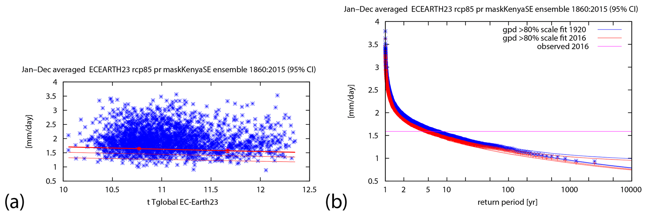
Figure 8 Similar to Fig. 4 but for the low precipitation event in the south-east of Kenya in 2016, using a GPD that scales with GMST and evaluated for the years 1920 and 2016. The figures show data of the 16 ensemble members of the EC-Earth model and the fit uses the lowest 20 % of the data. See Uhe et al. (2018) for more details.

If the model run extends into the future, the same method can be used to analyse the future scenario, for instance for a 2 ^∘C warmer world or the year 2050. With this a statement on the future can be made for this model. The standard approach is to compare the future to the current climate, for example, “According to model simulations used here, in a transient 2 ^∘C warmer world relative to pre-industrial, events similar to the extreme observed this year will be commonplace, occurring nearly every year”.

Finally, some model runs have been designed for comparisons between the current and a counterfactual climate but include transient runs to establish climatologies (e.g. weather@home, UK Met Office HadGEM3-A attribution runs). This enables both methods to be used for the same model, giving two estimates for the PR and ΔI that have independent confidence intervals due to internal variability.

7 Step 6: Hazard synthesis

The previous steps give different types of results for the same class of events: probability ratios and changes in intensity, for both observational data and model data (possibly based on different experimental framings). We now have to synthesize these partial results into a single attribution statement. This is an area of active research, and the methods discussed here are just the state of the art at this moment but will likely be improved upon in the near future. Current experiments using a new synthesis method with better theoretical justification give results comparable to those in Fig. 9.

First the fits to observations and transient runs have to be converted to a common baseline. For this we often take 1900, as it is often a good balance between the availability of observations and model runs and convenience in communicating results. However, this year annual observed GMST was about 0.1 ^∘C above the trend line for a 298.8 ppm CO₂ concentration and hence even more above true pre-industrial temperatures (Hawkins et al., 2017). If this year is not taken as a reference year in the fits, we can extrapolate back to 1900 using the same assumptions that were made in the fit, i.e. that the PDF shifts or scales with smoothed GMST (or another indicator of anthropogenic global warming). This also has to be done if we have (approximate) time slice experiments that start at a later date, e.g. RCM experiments starting in 1950. Next we assume that the effects of natural forcings were small over the last century, so that we can compare the 1900 results with the counterfactual world results. This is supported for global mean temperature by Bindoff et al. (2013) but is sometimes not true locally. Other local forcings such as aerosols, irrigation, and urban heat can also distort results.

Next the results are compared graphically, including 95 % uncertainties; see for instance Fig. 9. The differences between the values of the PRs and ΔI are due to natural variability, framings and model uncertainty. As the plotted uncertainties are only due to natural variability plus the model spread in multi-model ensembles, their importance relative to the other factors can be estimated. One way to do this is by computing a statistic that compares the spread in central values with their uncertainties: χ²∕dof, with the number of degrees of freedom, dof, 1 less than the number of fits. If this is roughly equal to 1, intra-ensemble variability (natural variability and the model spread of multi-model ensembles) dominates over framing and other model uncertainties. If it is much larger than one, the systematic differences among the model ensembles and between the ensembles and observations contribute significantly.

If the intra-ensemble variability dominates, which is often the case for precipitation, the final result can be obtained as a simple weighted average for PR and ΔI. This optimally reduces the noise. At the moment we assume that log (PR) is normally distributed and all results are independent as they have independent realizations of the natural variability. A refinement that may make sense is to treat lower and upper uncertainties separately if the uncertainty range from the bootstraps is asymmetrical, but more research is needed on this. An example is given in Fig. 9a. If we assumed the PDF shifts with the covariate, as for temperature, we also assume that ΔI is normally distributed. For a PDF that scales with the covariate, as for precipitation and wind, we take the exponential of the weighted average of log (ΔI).

If there is a significant contribution of χ² due to the spread of the different ensembles compared to their uncertainty estimates, the framing and model uncertainty do make a difference. If the framing affects the answer strongly the SST-forced experiments and coupled experiments should fall into two incompatible groups. In this case one should refine the attribution question (or split it into two questions) to either make it conditional on the relevant state of the ocean and only select coupled runs that agree with that or keep it general and add SST-forced experiments from other years. If this grouping is not apparent the spread is mainly due to model differences. This uncertainty has to be propagated to the final result and the final uncertainty is larger than the spread due to natural variability would indicate. One way to do this is to inflate the uncertainty by $\sqrt{{\mathit{\chi }}^{\mathrm{2}}/\mathrm{dof}}$. This method was used in Eden et al. (2016), van Oldenborgh et al. (2017), Philip et al. (2018c); see Fig. 9b for an example. We are currently trialling a mathematically better-defined method, which gives similar results.

Finally, if the observed and model trends are incompatible there is no way to synthesize the results (Fig. 9c and the only conclusion that can be drawn is that an attribution (or indeed projection) statement is not possible until all factors that caused the trend have been included realistically in the models.

Additionally, the comparison between modelled trends and observed trends serves as an extra model validation. If the response of extremes to external forcing is similar in observations and models, the confidence in the attribution results is higher. In case the response of extremes to external forcing is different in models and observations, no statement or an attribution statement only on part of the trend can be given. If this is the case, there is either the possibility of other forcings with trends that are not included in the models affecting the extremes (e.g. irrigation) or the models do not correctly represent the mechanisms leading to the extremes. In both cases the difference between models and observations can be useful input to model developers.

If the averaged (inflated) results for the PR and ΔI can be computed they are added to the bar plot with the observational and model results. This gives a strong visual check whether the synthesis makes sense.

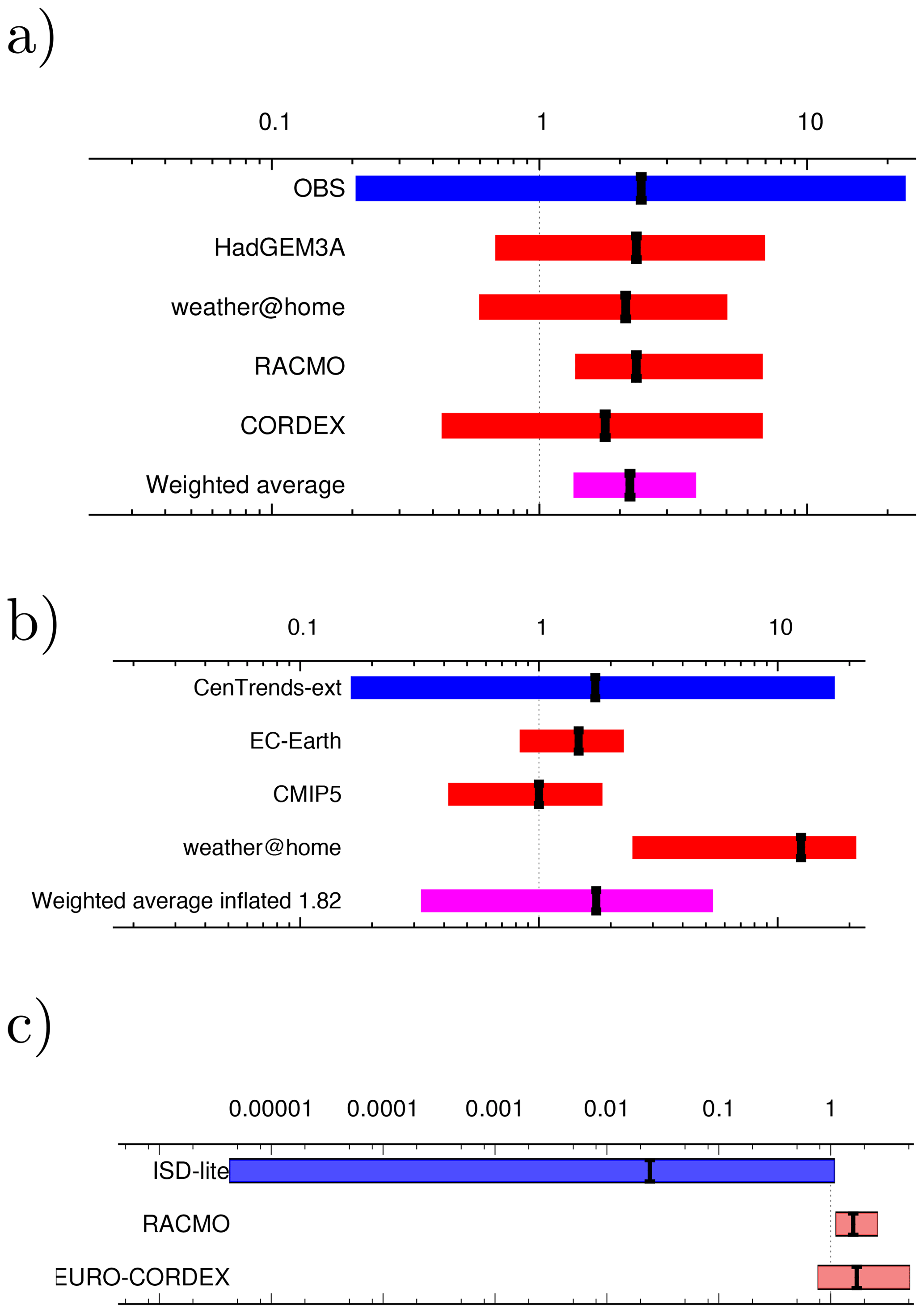
Figure 9 Synthesis plots of (a) the PR of extreme 3-day averaged precipitation in April–June averaged over the Seine basin (Philip et al., 2018b), (b) the PR of low precipitation in February–September in Ethiopia (8–13^∘ N, 38–43^∘ E) with inflated average (Philip et al., 2018c), and (c) the PR for changes in wind intensity over the region of storm Friederike on 18 January 2018 (after Vautard et al., 2019). Observations are shown in blue, models in red, and the average in purple.

If a statement on the future is given in the previous step for more than one model, a more general statement can be given here on the future as well. As the attribution analysis is often done as a function of the GMST, this can be extended easily to common transient warming scenarios that are formulated in the same terms: 1.5, 2 and 3 ^∘C above pre-industrial. Because often fewer values will be available for a synthesis on future probability ratios than for the synthesis of past probability ratios – not all models have future scenario runs or natural runs that continue into the future, and there is no probability ratio for the observed series – the values to be synthesized will be different from those for the past. To avoid erroneous direct comparisons with the synthesis result from observations and models on trends in the past, we recommend not to use the same synthesis method, rather make a more general statement. The temperature scenarios allow for statements like “As the planet continues to warm, at 2 ^∘C above pre-industrial this extreme would be expected to occur about X (Y to Z) more/less often than now.”

Note that probability ratios depend on the threshold used to define the event. Some extreme events, notably heat waves and to a lesser extent cold waves and droughts, follow an extreme value distribution with an upper limit (negative shape parameter) known as a reversed Weibull distribution. If the extremity of the event is such that it is found near this endpoint, small changes in the threshold result in large changes in return periods and probability ratios. The lower bound is then more stable and it may be preferable to emphasize it in communications. If, on the other hand, the distribution is modelled with a positive or near-zero shape parameter, which is usually the case for high precipitation events and low temperature events, then the probability ratio is less sensitive to small changes to the event threshold. This is useful to know if the threshold is uncertain due to lack of data of the event itself at the time of analysis.

8 Step 7: Vulnerability and exposure analysis

The synthesis above only concerns the probability of an extreme meteorological event. In risk terminology this is denoted by the term “hazard”. The overall risk is the product of hazard with two other terms: “exposure” and “vulnerability”. Exposure refers to the presence of people, livelihoods, infrastructure, and economic or social assets in places that could be adversely affected by extreme events. Vulnerability is the propensity or predisposition to be affected (Field et al., 2012). Vulnerability and exposure are key determinants of impacts when a risk is realized, underscoring the importance of including this information when communicating changing risks. There have been studies in which the total risk has been attributed to climate change Mitchell et al. (e.g. 2016); Schaller et al. (e.g. 2016), but these excluded trends in vulnerability and exposure. We find it advantageous to explicitly acknowledge these trends and do a quantitative attribution of the hazard (Sect. 7) plus a separate discussion of trends in vulnerability and exposure that is often qualitative.

When an attribution analysis is done because of the impacts (rather than a meteorological extreme with little impacts), an initial baseline of general, country-level vulnerability and exposure to different climate events is established through a review of existing metrics. Vulnerability and exposure are by definition characteristics that are specific to the location where the extreme event occurs and are characteristics that evolve over time, thus, the vulnerability and exposure analysis should be done in real time.

First, official disaster information from humanitarian, government networks, and media sources are reviewed to understand the impacts associated with the extreme event. Specifically who or what was impacted as well as when, where and how. This phase also informs the event definition (Sect. 3). With basic impact characteristics identified, we explore the wider context of why those specific impacts may have occurred.

Vulnerability and exposure data are often not uniform across countries, not updated, unavailable at resolutions other than country-level, or simply not collected. This makes it nearly impossible to have a standardized methodology for quantitatively assessing vulnerability and exposure in extreme events across many geographies. However, a few country-level standardized metrics do exist, for example the Inform Index, which provides a global, open source risk assessment and is now available at the sub-national level in eastern Africa.

A desk-based review is done of existing peer-reviewed literature, white papers and official reports from humanitarian institutions that provide insights into the drivers and characteristics of vulnerability and exposure related to the extreme event in the region. Characteristics can include a review of social, economic, geographic, demographic, cultural, institutional, governance and environmental factors. In a second stage, the trends in these factors are described, often only qualitatively. In-country stakeholders with knowledge or expertise in the specific vulnerability and exposure highlighted in the desk-based review are contacted to further inform the analysis. The inclusion of in-country partners both enhances our understanding and adds credibility to our communication. It is important to note that detailing the exposure and vulnerability context when an extreme event occurs is distinctly different from attempting to attribute the disaster impacts of an extreme event.

An example where the trends in vulnerability and exposure were found to be more important than the trends in the meteorological hazard is the attribution study of the drought in São Paulo (Otto et al., 2015). No trend was found in the hazard of low precipitation over the area feeding the city water system, but the large increase in the number of people using it and the increase in water consumption per person due to rising living standards had overtaken the capacity of the system leading to water shortages.

9 Step 8: Communication

The eighth and final step in the extreme event attribution analysis is the communication of the attribution statement. All communication operations require communication professionals. In this article we only describe the chain of communication of the analysis and synthesized results, omitting other types of communication that are not directly related to the analysis. Communication here concerns writing a scientific report, a more popular summary, targeted communication to policy makers, and a press release. We found that the first one is always essential; which of the other three are produced depends on the target audiences. The scientific report is key for traceability of numbers, data, and methods that will be communicated in other media. For all results it is crucial that during this chain the information is translated correctly into the different stages. This sounds obvious, but in practice it can be hard to achieve.

9.1 Scientific report

The scientific report details the procedure and intermediate results at a level that is sufficiently detailed such that another scientist can reproduce all results. This may be turned into a scientific article for peer review; however, a peer-reviewed paper is not always useful because the study may not be innovative. If the attribution study uses similar tools and data to earlier published analyses, it may not be worth the effort nor indeed be acceptable to scientific journals. However, if the procedures differ from peer-reviewed methods, new datasets have been used if unknown and different findings have been obtained, or the results are for an area where e.g. the existence of climate change is still widely debated in public discourse or, on the contrary, climate change is blamed falsely such that only a peer-reviewed study would carry enough weight, then this step is required. When pursuing peer review it is recommended to publish in an open-access journal to ensure maximum accessibility to the findings.

The purpose of the scientific report is 2-fold. Firstly, it is for transparency, such that people can check assumptions, event definition, and other decisions during the analysis. Secondly, when written alongside the analysis, the science report helps to improve communication within the analysis team as it provides a reference for all members to construct other communication forms.

9.2 Scientific summary

Next, a summary of the findings in 1 or 2 pages is written by those carrying out the analysis with input from communications partners. This summary is aimed at a scientifically literate public such as science journalists or scientists who want an accurate description of the results but have no need to reproduce the whole analysis. It needs to be concise but precise, including numbers and uncertainty ranges. It should cover a description of the event and impacts, the event definition, return period, model evaluation, separate model results, the synthesized attribution statement, and a summary of the vulnerability and exposure analysis. It is often useful to briefly mention how this analysis fits with other studies.

9.3 Policy-relevant summary

Similarly, a 1-page summary in non-scientific language may be prepared for local disaster managers, policy makers, and journalists with the impacts, the attribution statement, and the vulnerability and exposure analysis, preferably with the outlook to the future if available. The local team members and other stakeholders in the analysis can be invited to be points of contact for anyone seeking further clarification of contextual information, or they may be brought closer into the project team to collaborate and communicate key attribution findings.

Figure 10 Graphic designed by Climate Central for the November–December 2016 North Pole warmth attribution analysis, with changes in intensity and probability visualized for the past, present, and future. From van Oldenborgh et al. (2016a).

9.4 Press release

A press release may be written by communications partners. The press release should contain understandable common language. Furthermore, we found that after inserting quotes from the scientists that performed the analysis, people gain more confidence in the results. This may include accessible graphics, such as the representation of the change in intensity and probability of very mild months in the high Arctic as observed in November–December 2016 in Fig. 10 (van Oldenborgh et al., 2016a).

9.5 Social media

Finally, social media can be used to amplify the spread of attribution findings and contribute to public discourse on the extreme event being studied. Social media can also help to reach younger audiences (Hermida et al., 2012; Shearer and Grieco, 2019; Ye et al., 2017). Social media monitoring and analytics can also be used to assess awareness and the spread of attribution findings (Kam et al., 2019).

9.6 Automation

Some of the outreach products can also be generated automatically on a website that progressively reveals more and more information, as currently being trialled by the UK Met Office as part of the European project EUPHEME. At the moment this is in the prototype stage and so only covers part of the methodology: only a single model and only the event definition step (given by the user) and attribution steps. It is possible that such a design will generate or supplement some of the hand-made products described above in the future.

9.7 Different outcomes

In attributing an extreme event to anthropogenic climate change, four different outcomes are possible. The communication step is simplified if templates are available for all outcomes.

• (i)

  The event was made more likely due to anthropogenic climate change.

• (ii)

  The event was made less likely due to anthropogenic climate change.

• (iii)

  Anthropogenic climate change did not alter the frequency of occurrence of the event.

• (iv)

  With our current understanding and tools we cannot assess whether and how the event was influenced by anthropogenic climate change.

Awareness of these outcomes, and their implications, is important, especially if the outcome aligns with the fourth category. Regardless of the results, it is important to maintain a consistent level of effort to communicate the results, otherwise there is a risk of creating a positive communication bias, as in much scientific literature. Positive results are more frequently written up than negative results in peer-reviewed journals and high-profile journals reject negative results out of hand.

Examples of these four different types of outcomes are listed below.

• (i)

  The conclusion of the analysis of the extreme precipitation in southern Louisiana in August 2017 by van der Wiel et al. (2017) was that anthropogenic climate change made such an event more likely; they found that there is a significant increase in probability of a factor of 2.8 (95 % CI 1.7 to 3.8).

• (ii)

  The analysis of the cold wave in June–August 2013 in Peru by Otto et al. (2018b) leads to the conclusion that such an event has become less likely due to climate change. In the past, such cold events happened more often: the probability ratio is 0.08 (95 % CI 0.02 to 0.21).

• (iii)

  In the analysis of Philip et al. (2018c) on the Ethiopian drought of 2015, taking the model spread into account they cannot attribute the drought to anthropogenic climate change, with the 95 % confidence interval ranging from a probability decrease between pre-industrial and now of a factor 0.3 and an increase of a factor 5. Increases or decreases larger than this can however be excluded.

• (iv)

  The analysis of the area averaged temperature anomaly of the Mediterranean heat wave in 2017 did not lead to an answer to the attribution question in Kew et al. (2019). The conclusion of this analysis was that although they cannot give an attribution statement based on both observations and model analyses, from observations it is clear that there is a positive trend in the occurrence of hot events like the heat wave in August 2017. Observations show that since 1950 the risk has at least quintupled, but is probably much higher.

9.8 Language

There has been some research into the efficacy of different ways to communicate results and uncertainties to a large audience. For instance, van der Bles et al. (2018) found that a numerical uncertainty range hardly decreases trust in a statement, whereas a language qualification does decrease it significantly. We also found that communicating only a lower bound, because it is mathematically better defined in many cases, is not advisable. In the first place a phrase like “at least” was found to be dropped in the majority of popular accounts. Secondly, quoting only the lower bound de-emphasizes the most likely result and therefore communicates too conservative an estimate (Lewandowsky et al., 2015).

10 Conclusions

In this paper we have written down the detailed methodology of extreme event attribution as developed and used by WWA and that can be deployed in an operational near-real-time attribution service. The eight steps of this method have been set up and polished during rapid and slower attribution studies. Analyses performed by WWA show that the protocol is practical and helps to streamline attribution studies of extreme events.

As methods develop, this protocol may no longer be complete and the method can be complemented when new insights are gained. It is not meant to exclude other methods. It is, however, a method that has already been tested in rapid and slower analyses, and verified by additional validation studies (Otto et al., 2018a; Philip et al., 2018b). It is thus ready for use in extreme event analyses, including rapid analyses, and by operational services. More research is needed in particular steps in our framework, such as in refining the validation of climate models and the synthesis of results. These topics are currently being addressed within the European project EUPHEME.

Other methods that are currently being developed and tested could complement the ones described in this paper in the future. For communication purposes the storylines approaches could fit well and theoretically be placed under a common framework with probabilistic approaches.