the Creative Commons Attribution 4.0 License.
the Creative Commons Attribution 4.0 License.
 | 14 Dec 2022
Evaluation of simulated responses to climate forcings: a flexible statistical framework using confirmatory factor analysis and structural equation modelling – Part 1: Theory
Katarina Lashgari
Gudrun Brattström
Anders Moberg
Rolf Sundberg
Evaluation of climate model simulations is a crucial task in climate research. Here, a new statistical framework is proposed for evaluation of simulated temperature responses to climate forcings against temperature reconstructions derived from climate proxy data for the last millennium. The framework includes two types of statistical models, each of which is based on the concept of latent (unobservable) variables: confirmatory factor analysis (CFA) models and structural equation modelling (SEM) models. Each statistical model presented is developed for use with data from a single region, which can be of any size. The ideas behind the framework arose partly from a statistical model used in many detection and attribution (D&A) studies. Focusing on climatological characteristics of five specific forcings of natural and anthropogenic origin, the present work theoretically motivates an extension of the statistical model used in D&A studies to CFA and SEM models, which allow, for example, for non-climatic noise in observational data without assuming the additivity of the forcing effects. The application of the ideas of CFA is exemplified in a small numerical study, whose aim was to check the assumptions typically placed on ensembles of climate model simulations when constructing mean sequences. The result of this study indicated that some ensembles for some regions may not satisfy the assumptions in question.
- Article
(1778 KB) - Full-text XML
- Companion paper
-
Supplement
(983 KB) - BibTeX
- EndNote


Climate models are powerful tools used for investigating how the climate system works, for making scenarios of the future climate and for assessing potential impacts of climatic changes (Flato et al., 2013). Using a numerical representation of the real climate system, climate models are designed as systems of complex differential equations based on physical, biological, and chemical principles. In the virtual world of climate models, scientists can perform experiments that are not feasible in the real world climate system. For example, one can neglect or simplify all but one process, in order to identify the role of this particular process clearly, for example, the influence of changes in solar irradiance on the radiative properties of the atmosphere, or to test hypotheses related to this process. In an analogous fashion, the overall effect of several processes, acting jointly, can be investigated.
In order to assess the magnitude of the effects of the processes in question on the climate, it is often convenient to analyse their impact on the radiative balance of the Earth (Goosse, 2015). The net change in the Earth's radiative balance at the tropopause (incoming energy flux minus outgoing energy flux expressed in watts per square metre (W m−2)) caused by a change in a climate driver is called a radiative forcing (see, for example, Myhre et al., 2013; Liepert, 2010). Sometimes scientists use the term climate forcing instead of radiative forcing (Liepert, 2010). We will generally do so in our discussion, or we simply write just forcing.
Examples of external natural drivers of climate change, which are capable of inducing climate forcing, are changes in solar radiation, changes in the orbital parameters of the Earth, and volcanic eruptions. There are also external drivers of climate change of anthropogenic origin, for example, the ongoing release of carbon dioxide to the atmosphere, primarily by burning fossil fuels, the emissions of aerosols through various industrial and burning processes, and changes in land use (Jungclaus et al., 2017). Climate variability can also be caused by various processes internal to the climate system itself (Kutzbach, 1976). Ocean and atmosphere circulation and their variations and mutual interactions are examples of processes that are clearly internal to the climate system.
The range of types of climate models is very wide. Here, our focus is on the most sophisticated state-of-the art climate models referred to as global climate models (GCMs) or Earth system models (ESMs). As computing capabilities have evolved during the past decades, the complexity of GCMs and ESMs has substantially increased: for instance, the number of components of the Earth system that can be included and coupled in GCMs and ESMs has increased, or the previously often performed equilibrium simulations can now be replaced by transient simulations, driven, for example, by temporal changes in the atmospheric greenhouse gases (GHGs) and aerosol loading (see, for example, Cubash et al., 2013; Eyring et al., 2016; McGuffie and Henderson-Sellers, 2014; Jungclaus et al., 2017).
However, despite great advances achieved during the past decades, some simplifications are unavoidable, for example, due to the range of temporal and spatial scales involved and/or incomplete knowledge about some processes. As a consequence, the complexity of the most sophisticated climate models is still far from the complexity of the real climate system. Even a careful design cannot guarantee that each component of climate modelling, for example, parameterisation of subgrid-scale processes, has been employed in its optimal form. Also, our knowledge about various feedback processes, for example, cloud feedback (Gettelman, 2016), that may either amplify or damp the direct effect of a given forcing is not complete.
Another type of complication is that forcing reconstructions too may be uncertain. As examples, uncertainties can be large for such anthropogenic forcings as aerosol forcing and land use forcing (Hegerl and Zwiers, 2011), and the amplitude of natural solar irradiance changes in the last millennium has been disputed (Feulner, 2011).
All the above-mentioned issues together point naturally to the importance of carefully undertaking evaluation of climate model simulations by comparison against the observed climate state and variability. An important role in this context has been played by so-called detection and attribution (D&A) studies (e.g., Hegerl et al., 2007, 2010; Mitchell et al., 2001; Santer et al., 2018; Wigley et al., 1990). Within these studies, the question of attribution of observed climate change to real-world forcings is addressed simultaneously with the question of consistency between simulated and observed climate change. That is, one of the goals of D&A studies is to evaluate the ability of forced climate models to simulate observed climate change correctly.
Based on the ideas of Hasselmann (1979), statistical methods used in D&A studies performed to date have been given different representations (Hasselmann, 1993, 1997; Levine and Berliner, 1998) and typically are referred to as “optimal fingerprinting” techniques. In the present work, the focus is on the representation associated with linear regression models, described by Allen and Stott (2003).
In terms of the near-surface temperature, which has been a climatic variable of interest in many D&A studies, an advantageous assumption made in Allen and Stott (2003) is that neither the real temperature responses to particular forcings, nor the simulated responses to imposed forcings obtained in experiments with complex GCMs or ESMs are directly observable; that is, they are latent. This has motivated the use of regression models with latent variables where both explanatory and response variables are contaminated with noise. In the statistical literature, these regression models are known as measurement error (ME) models (sometimes also-called errors-in-variables models).
Being the simplest model among statistical models with latent variables, the ME model specification has proved to be a useful tool within many D&A studies that greatly contributed to the understanding of the causes of climate variability. However, as recognised by several researchers, this statistical model is associated with certain limitations, for example, the inability to take into account the effects of possible interactions between forcings (see, for example, Marvel et al., 2015; Schurer et al., 2014) or the inability to account for non-climatic noise in the observational data.1 Nor does the simplicity of the ME model specification allow researchers to avoid the estimation issues that arise under the so-called “weak-signal” regime (DelSole et al., 2019) or to specify more complex latent structures for data that are supposed to contain signals associated with complicated climatological feedback mechanisms, for example, climate–vegetation interactions.
Having a statistical framework that can address the questions posed in the D&A studies and, at the same time, lends itself to flexible specifications of latent structures, depending on hypotheses that researchers have and on the properties of both the climate model and the forcings considered, may potentially aid in overcoming the above-mentioned limitations of the ME model. All these points together may ultimately increase our confidence in the final estimates and conclusions drawn.
The goal of the present study is to formulate such a statistical framework by investigating possible extensions of the ME model specification to more complex statistical models with latent variables.
To this end, we used the fact that a ME model is a special case of a confirmatory factor analysis (CFA) model, which in turn is a special case of a structural equation modelling (SEM) model (Jöreskog and Sörbom, 1989). Regarding the relationships between model variables, the differences between these three types of statistical models are as follows:
-
ME model. Only latent variables are allowed to influence their observable indicators. Latent variables can be related to each other only through correlations. All latent variables are assumed to be correlated.
-
CFA model. This is as a ME model above, but it is possible to introduce restrictions on model parameters, for example, zero correlations.
-
SEM model (standard representation). Latent variables may influence not only observable variables, but also each other (either unidirectionally or reciprocally). That is, latent variables may be related to each other not only through correlations, but also through causal relationships, modelled by means of regression models.
-
SEM model (alternative representation). This is as a standard SEM model above. In addition, observable variables are also allowed to influence latent variables.
As a matter of fact, the notion of causality is not new to climate research. As examples, we can refer to Kodra et al. (2016) and Stips et al. (2016), where the causal structure between atmospheric CO2, i.e. the forcing itself, and global temperature has been studied by applying the methods based on Granger causality and the concept of information flow, respectively. The latter concept was also used by Liang (2014) to investigate the cause–effect relation between the two climate circulation dynamic modes, El Niño and the Indian Ocean Dipole. But our questions to be addressed here and the methods we use for achieving our goals are different compared to the works mentioned above.2
When formulating CFA and SEM models here, we also used the ideas of another statistical framework developed by Sundberg et al. (2012) (hereafter referred to as SUN12). The SUN12 framework, which has so far only been used in just a few studies (Hind et al., 2012; Hind and Moberg, 2013; Moberg et al., 2015; PAGES2k-PMIP3 group, 2015; Fetisova, 2015), was designed to suit the comparison of climate model simulations and temperature reconstructions derived from climate proxy data for the last about 1 millennium. As the main result, SUN12 formulated two test statistics: a correlation and a distance-based test statistic, each of which is based on one and the same ME model with a single latent variable. Although SUN12, just as D&A studies, uses the ME model specification, this framework has suggested another approach of relating simulated temperatures to observational data in terms of common latent factors. The approach suggested, in our opinion, may enable the attribution of observed climate change without simultaneous testing of the consistency between simulated and observed climate change.
The statistical models considered here are intended to be suitable for the type of observational and climate model data that is typically available for the last millennium, as also exemplified in some D&A studies (e.g. Hegerl et al., 2011; PAGES2k-PMIP3 group, 2015; Schurer et al., 2013, 2014). Nevertheless, the concepts proposed here are based on general theory, and our ideas may therefore also be extended and adapted for being used with modern data, like in most D&A studies.
Finally, let us describe the structure of the present paper. First, in Sect. 2, some main assumptions and
definitions of our framework will be described. Section 3 gives an overview of the statistical model
used in D&A studies and its link to the CFA model specification.
Section 4 provides a description of our CFA models, while the SEM models are presented in Sect. 5.
Section 6 provides a brief practical demonstration of fitting a simple CFA model to two ensembles of climate
model simulations using the R package sem.
The paper is concluded by an overview of the key characteristics of all the statistical models presented
(see Sect. 7).
2.1 Near-surface temperature
Although both the real and simulated climate systems comprise several climate variables in a 3-dimensional spatial framework in the atmosphere, in the oceans, and on land, here we will only think in terms of air temperatures near the Earth's surface. Climate scientists often refer to this as either surface air temperature or 2 m air temperature depending on context. We will simply call this “temperature”.
2.2 Unforced versus forced climate models
The term “unforced climate model” or just “unforced model” denotes here a simulation not driven by any external forcing. That is, only internal factors influence the simulated temperature variations. More precisely, the boundary conditions that are associated with the forcing factors of interest are held constant throughout the entire simulation time, at some level selected by the researcher. Climate modellers often refer to this kind of simulation as a control simulation.
When running the same climate model again, but with the control boundary conditions replaced with a reconstruction
of temporal and spatial changes in a particular forcing f, one obtains a forced climate model simulation.
Climate modellers sometimes refer to this situation as a transient model simulation, while we refer to it as
a “forced climate model” or just “forced model”.
2.3 Specifying forcings of interest
To make our way of reasoning as clear and concrete as possible, we focus on five specific forcings:
-
changes in the solar irradiance (abbr. Sol);
-
changes in the orbital parameters of the Earth (abbr. Orb);
-
changes in the amount of stratospheric aerosols of volcanic origin (abbr. Volc);
-
changes in vegetation and land cover caused by natural and anthropogenic factors (abbr. Land);
-
changes in the concentrations of greenhouse gases in the atmosphere (abbr. GHGs), also of both natural and anthropogenic origin.
In the real-world climate system within a certain region and time period t, , these forcings generate the corresponding latent true temperature responses, which we denote as follows3: , , , , and . Note that due to the properties of the Land and GHG forcings, and are defined as overall true temperature responses, each of which contains two components, representing temperature responses to natural respectively anthropogenic changes. Importantly, we regard anthropogenic changes, caused by human activity, as physically independent processes of the natural forcings (we do not discuss here any possible influence of the changed climate on the actions of humanity).
All the above-specified forcings are identified as drivers of the climate change during the last millennium (Jungclaus et al., 2017). Therefore, state-of-the-art Earth system model (ESM) simulations driven by these (or some of these) forcings both individually and jointly are already available (Otto-Bliesner et al., 2016; Jungclaus et al., 2017), thereby making the issue of their evaluation relevant.
Depending on the scientific question of interest, climate models may be driven by different combinations of reconstructed forcings. For the purpose of our theoretical discussion, let us first assume that the following temperature data from climate model simulations are available:
- {xSol t}
-
is forced by the reconstruction of the solar forcing, which generates the simulated counterpart to , denoted4 .
- {xOrb t}
-
is forced by the reconstruction of the orbital forcing, which generates the simulated counterpart to , denoted .
- {xVolc t}
-
is forced by the reconstruction of the volcanic forcing, which generates the simulated counterpart to , denoted .
- {xLand t}
-
is forced by the reconstruction of the Land forcing of both natural and anthropogenic origin, which generates the two-component simulated counterpart to , i.e. . In contrast to anthropogenic changes in land cover, which are reconstructed, natural changes in vegetation can be simulated in climate models by involving dynamic land vegetation models. In practice, this means that climate model simulations driven only by the reconstructed anthropogenic land-use forcing or only by natural changes in vegetation can be available.
- {xGHG t}
-
is forced by the reconstruction of the GHG forcing of both natural and anthropogenic origin, which generates . Unlike the Land forcing, the GHG forcing is not assumed to possess available climate model simulations driven only by natural changes in the forcing.
- {xcomb t}
-
is forced by all reconstructed forcings above, generating the overall simulated temperature response .
Note that we do not assume that climate model simulations driven by all possible combinations of forcings, for example, the combination of solar and volcanic forcings or the combination of solar and Land forcing, are available.
A general statistical model, used for assessing the individual contribution of m forcings in many D&A studies made after 2003, is given by the following ME model with a vector explanatory variable (see, for example, Allen and Stott, 2003; Huntingford et al., 2006; Schurer et al., 2014):
where yg is the mean-centred observed/reconstructed temperature, where the index g reflects the fact that the {yg} sequence is allowed to be a temperature field, arrayed in space and in time; xi g is the mean-centred simulated temperature, generated by the climate model forced only by a reconstruction of forcing i; νi g is the simulated internal temperature variability associated with the climate model driven by forcing i; ν0 g is the real internal temperature variability, i.e. the real latent unforced component embedded in yg; xi g−νi g is the simulated latent temperature response to forcing i, embedded in xi g; and βi is a scaling factor associated with forcing i.
For the purpose of our analysis let us rewrite model (1) with respect to the specified forcings and partly by using our notations. Moreover, realising that the ME model in the form presented does not take into account the initial space-time dimensionality of data but simply presupposes that each model variable is associated with a single vector of values of the same length across all variables, we replace the subindex g by the subindex t, representing the time point t, . So for the time point t and any region, we get the following model:
where f ranges over .
In statistical literature, this kind of a ME model is
known as a ME model with no error in the equation (see, for example, Fuller, 1987; Cheng and van Ness, 1999). To enable the inferences,
one typically assumes that the error vectors are normally
and independently distributed under a wide range of distributional assumptions for .
Also, one assumes that the errors are uncorrelated with , associated in their turn
with a non-singular variance–covariance matrix.
In the case of Eq. (2), the term “no error in the equation” refers to the fact that the overall true temperature response to all forcings, acting in the real-world climate system and embedded in yt, is modelled as an error-free linear function of the five simulated temperature responses of interest, that is
where f ranges over , and
is our notation for the overall true temperature response to all forcings acting
in the real-world climate system. From Eq. (3), it also follows that for each individual
forcing f,
where is a real-world counterpart to .
Equations (3) and (4) are justified by the assumption, made in D&A studies, that the (large-scale) shape of the true temperature response is correctly simulated by the climate model under consideration (see, for example, Hegerl et al., 2007; Hegerl and Zwiers, 2011). Hence, we may say that model (2) assumes that the simulated temperature response can differ from the corresponding only in its magnitude, represented by the parameter β𝚏.
The introduction of an error into Eq. (3) would entail another structure of the variable representing the random variability in yt. In other words, ν0 t would only be a part of the random component of yt. The structure of the random component may be even more complex if one wishes to take into account a non-climatic noise, which can constitute quite a large part of temperatures reconstructed from proxy data (Hegerl et al., 2007; Jones et al., 2009) and which can also exist in varying amounts in instrumental temperature observations (Brohan et al., 2006; Morice et al., 2012). According to Allen and Stott (2003), the main reason for excluding the corresponding error term, known as observation error, is that its autocorrelation structure is assumed to differ from that associated with the internal temperature variability.
From the estimation point of view, a consequence of adding various error terms to ν0 is that one may need to use another estimator of β𝚏s instead of that used in D&A studies. The estimator used is known as the total least squares (TLS) estimator, and it requires the knowledge of the ratios of the variances of ν𝚏 and ν0, which can be quite challenging to derive if ν0 is replaced by a multi-component variable.
Importantly, the TLS estimator remains unchanged if the whole error variance–covariance matrix is known a priori. In practice, this knowledge permits us to check for model validity, provided one derives this a priori knowledge from a source independent of the sample variance–covariance matrix of the observed variables. In D&A studies, such a source is unforced (control) climate model simulations.
We would also like to emphasise the fact that the TLS estimator is obtained under the condition that all latent variables are correlated. This entails that if some s are highly mutually correlated or at least one of s does not vary much, unreliable estimates are expected. Thus, it is important to check whether the variance–covariance matrix of the latent variables is singular or not.
The main parameters of interest, estimated within D&A studies, are the coefficients β𝚏. They are involved in two important hypotheses. The first one concerns the detection of the corresponding simulated temperature response in the observed climate record yt. The rejection of H0: β𝚏=0 indicates that is detected in yt. The rejection also indicates the so-called “strong-signal regime” (DelSole et al., 2019), associated with high reliability of all the parameter estimates and their associated confidence intervals (provided, of course, the variance–covariance matrix of latent variables is still non-singular).
The detection of a simulated temperature response, however, in the observed climate record is not
sufficient for attributing this detected simulated temperature signal to the corresponding
real-world forcing f. For this, one needs to show that is consistent
with , i.e., that Eq. (4) holds with
β𝚏=1. Thus, the second hypothesis of interest in D&A studies is
H0: β𝚏=1, known as the hypothesis of consistency.
However, as emphasised by Hegerl et al. (2007),
the test for consistency, referred to by the authors as “attribution consistency test”, does not constitute
a complete attribution assessment, though it contributes important evidence to such an assessment.
Another important feature of model (2) is that it does not take into account the effect of possible interaction(s) between forcings. Instead, the model assumes the additivity of forcing effects. The issue of additivity has been recognised and discussed by many researchers within the D&A field. Several analyses have been performed to investigate the significance of interactions in simulated climate systems (see, for example, Gillett et al., 2004b; Marvel et al., 2015; Schurer et al., 2014). The results seem to support the assumption of additivity when it concerns temperature. Nevertheless, it would be beneficial to develop a statistical model permitting a simultaneous assessment of the magnitude of both individual and interaction effects of forcings on temperature.
Summarising the overview above, we may say that it is highly motivating to investigate possibilities of extending the ME model representation to more complex statistical models in order to overcome the limitations of the ME model.
To achieve this aim, we suggest using the close link between ME, CFA, and SEM models. To see that the ME model in Eq. (2) can be viewed as a CFA model, let us first rewrite this model in the matrix form as shown in Eq. (5).
In the matrix form given in Eq. (5), the ME model is represented as
an unstandardised CFA model, that is, a CFA model with unstandardised latent factors.
The pattern of the model coefficients, also-called factor loadings in CFA literature, reflects our
conviction that observations on x𝚏 were generated by the climate model driven only by forcing f.
In other words, model (5) tells us that
each x𝚏 t only has one common latent factor with yt, that is .
Note also that an unstandardised factor model is associated with an unstandardised solution. However, a standardised solution is preferred because its model coefficients (hereafter called standardised coefficients) make it possible to judge the relative importance of latent factors. The standardisation of the latent factors in model (5) is accomplished by standardising their variances to 1. The resulting CFA model is given in Eq. (6). Since the model has been derived from a ME model, we call model (6) a six-indicator and five-factor ME-CFA model, abbr. ME-CFA(6, 5) model.
In model (6), the ratio
gives us back β𝚏, associated with the ME model in Eq. (2),
for each forcing f. Thus, the hypotheses concerning β𝚏 are applicable to
the parameters κ𝚏 and α𝚏. In particular, the hypothesis
H0: β𝚏=0 corresponds to H0: κ𝚏=0, while the hypothesis of
consistency is equivalent to H0: or equivalently H0: κ𝚏=α𝚏.
In practice, it is not difficult to test various equality constraints within a CFA model – one simply fits the associated factor model under the constraints of interest. That is, one fits and tests simultaneously (for more theoretical details about the estimation of CFA models, see the Appendix). In the same manner, one may introduce restrictions on the correlations among the latent factors.
where ,
, and ,
for each forcing f.
Another advantage of thinking in the spirit of CFA is that the factor model specification makes it possible to take into account the lack of additivity, which may arise due to possible interactions between forcing. This can be accomplished by adding observable variables associated with various multi-forcing climate model simulations (provided such simulations are available). Finally, this model specification seems to permit a complete attribution assessment, provided one uses s as common factors instead of s.
In this section, our aim is to formulate a basic CFA model with respect to the five specified forcings. The model is called basic because it is supposed to be modified depending on the climate-relevant characteristics of the specified forcings for the region and period of interest. Note also that we focus on a CFA model with standardised latent factors in order to enable meaningful comparisons of estimated effects of latent factors. For a brief account of general CFA models and the associated definitions, used in the following sections, see the Appendix.
As mentioned in the Introduction, one of the starting points for our framework is the SUN12 framework. Within the confines of the present work, we combine some of the definitions in SUN12 that are relevant for our work with our definitions.
Like D&A studies, decomposing the climate variability within the ME model into forced and unforced components, SUN12 also implements the same decomposition within its statistical model. However, unlike D&A studies, SUN12 allows more complex structures of random components both in yt and in x𝚏. Using this feature of SUN12, our initial model for the mean-centred yt for a given region and time t, , is as follows:
where the forced component was defined in Eq. (3), and the random component , assumed to be independent of , contains, for each t, (1) the internal random variability of the real-world climate system, including any random variability due to the presence of the forcings, and (2) the non-climatic noise. Although SUN12 allows the non-climatic variability to vary depending on the time period, in this work, for simplicity, we will assume that the variance of is constant for each time point.
Since there are five forcings under investigation, the next step is to rewrite yt in Eq. (7) under the assumption that only these five true forcings may systematically contribute to the variability in yt. In doing so, we also want to allow a term for the lack of additivity, due to possible interactions between the forcings. The resulting equation is as follows:
where (i) denotes the overall temperature response to all possible interactions between the forcings under consideration; (ii) the parameters Strue, Otrue, and so on are standardised coefficients, denoting the magnitude of the individual contribution from the associated real-world forced processes to the variability in yt; and (iii) , assumed to be independent of all s in the equation, represents residual variability arising after extracting the six specified true temperature responses from . As one can see, the random component νt in Eq. (8) has a more complex structure than the corresponding random component ν0 t in model Eq. (2).
In a similar way, our initial model for x𝚏 t is given by
where was defined in Sect. 2, and
, assumed to be independent of , represents the simulated
internal random temperature variability, including any random variability due to the presence of
the forcing f.
Hence, Eq. (9) does not require the same random variability for forced climate model simulations
generated by the climate model under consideration when it is driven by different forcings.
The next step is to rewrite each x𝚏 t as a function of the corresponding . The idea of modelling true temperature responses as common factors for x𝚏 t and yt was suggested in SUN12 but without exploring its consequences. Here, it should be realised that the replacement of s by corresponding s is not only a question of different notation. This replacement entails different structures and interpretations of error terms, called specific factors in CFA literature. As a result, different factor models arise.
Let us describe this process by example of xSol t. The extraction of from leads to the following equation:
where the residual term , assumed to be independent of , arises as a result of extracting from and is supposed to represent the large-scale shape of . Further, the coefficient Ssim reflects the idea that the magnitude of the common factor , extracted from , is not necessarily the same as its true magnitude, represented by the coefficient Strue in Eq. (8).
Assuming that both magnitude and the large-scale shape of the true temperature response are correctly simulated, Eq. (10) transforms to
Thus, the meaning of the consistency within our framework is that a simulated temperature response can be represented as an error-free function of the corresponding real-world temperature response with the same magnitude as that observed in yt.
An important feature of our framework is that it involves x comb as an additional observable variable, assumed to contain the simulated counterparts to each and to . Our initial model for x comb t is
which after extracting the six true temperature responses from transforms to
Notice that each in Eq. (13) is associated with the same
coefficient as that representing the magnitude of within x𝚏 t
(see, for example, Eq. 10). These equalities are justified by the fact that the underlying
, embedded in x𝚏 and in x comb, has been generated by
the same implementation of forcing f and that the same climate model is used in both cases.
Statistically, this repeatedness of each allows us to treat them
(and s as well) as a repeatable outcome of random variables, each of which is assumed to
be normally and independently distributed with zero mean and its own variance.
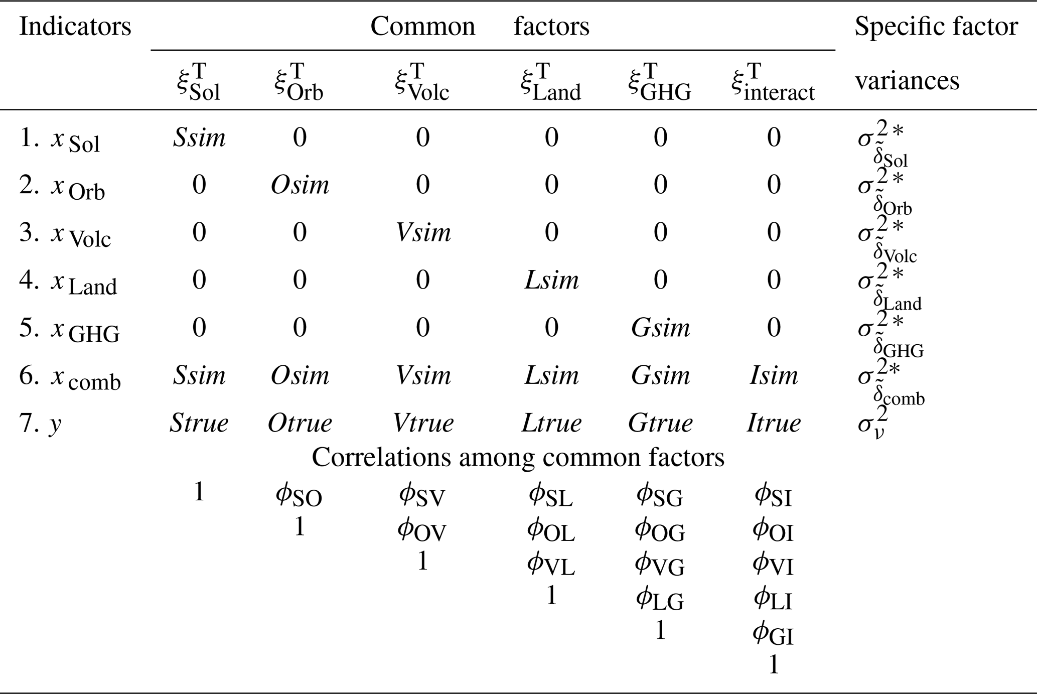
Table 1Parameters of the seven-indicator and six-factor model, abbr. CFA(7, 6) model, hypothesising the consistency and the uncorrelatedness between three latent factors.

∗ The parameter assumed to be known a priori.
It is also important to highlight that under the CFA (and ME) model specification, all common latent factors can be related to each other only through correlations. Climatologically, this corresponds to viewing all underlying forcings as physically independent processes not capable of causing changes in each other but giving rise to temperature responses that can be either mutually correlated or not.
Given the preliminaries above, we can finally formulate our basic CFA model that hypothesises the consistency between the simulated and true temperature responses. The parameters of the resulting CFA model with seven indicators and six common factors are given in Table 1. Importantly, the CFA model presented hypothesises not only the consistency, but also zero correlation between , , and . Our motive for these zero correlations is that the forcings that generate these temperature responses are acting on different timescales and with different character of their temporal evolutions. It is thus reasonable to expect that their temperature responses will not demonstrate a similar temporal pattern. On the other hand, we find it difficult to hypothesise zero correlations between and , , and . Thus each of the last three responses is allowed to be correlated with .
Another feature of the model is that the variances of the specific factors s, where f represents either one of the individual forcings or their combination,
are treated as known a priori, i.e. as fixed parameters.
To obtain an a priori estimate of each , we suggest using the following estimator
if the x𝚏 ensemble of interest contains at least two members or replicates:
where is the average of the observations at time t. In case it is climatologically justified to assume that the forcing of interest has a negligible influence on the temperature variability, one can use instead the sample variance of all nk𝚏 observations, i.e.
where is the average of all observations. In Sect. 6, we discuss the assumptions associated with the estimators above and demonstrate in practice how these assumptions may be checked using the ideas of CFA.
The advantage of treating s as fixed parameters is that it enables the estimation, i.e. identifiability, of a CFA model without hypothesising the consistency for each and the uncorrelatedness between , , and (in case the latter is climatologically motivated for the region and period of study). The resulting CFA model is given in Table 2. This CFA model is just-identified with 0 degrees of freedom. As a consequence, it is not possible (and unmotivated) to test for lack of fit to the data.
In contrast, the CFA model in Table 1 is over-identified with 9 degrees of freedom, which makes it meaningful to test whether the empirical data conform to the hypothesised latent structure. If all the estimates of this CFA model are admissible and interpretable, and if the model fits the data adequately both statistically or heuristically (see Eqs. A5–A8 in the Appendix), then one may say that there is no reason to reject the hypotheses that both magnitude and shape of the simulated temperature response are correctly simulated by the climate model under consideration.
In addition, the estimates of the factor loadings can be used for assessing the contribution of the real-world forcings to the variability in yt. For example, provided that the parameter estimates of the CFA model in Table 2 are admissible and climatologically interpretable, the rejection of H0: Strue=0 indicates that the true temperature response to the real-world solar forcing is detected in observational data. That is, the attribution to the real-world forcings is possible, even if the hypothesis of consistency is relaxed.
Both above-presented CFA(7, 6) models can be modified by setting desirable and climatologically justified constraints on the parameters. For example, for testing that the effect of interactions is negligible, one needs to set Itrue (and Isim, depending on which CFA model is considered) to zero. Importantly, one also needs to set each of the five associated correlations to zero in order to avoid under-identifiability. As a result, one gains 6 additional degrees of freedom if the over-identified CFA model from Table 1 is analysed. In the case of the CFA model from Table 2, the zero constraints imposed makes the model over-identified with 7 degrees of freedom.
Similar constraints can be placed on the parameters associated with other common factors, if one expects negligible forcing effects for the region of interest. Otherwise, the estimation procedure may become unstable, which may lead to an inadmissible solution or even the failure to converge to a solution.
Another reason to modify the CFA models presented arises when instead of xLand climate model simulations only xLand (anthr) or xLand (natural) climate model simulations are available. When replacing the indicator xLand by xLand (anthr) or xLand (natural), one needs to replace the common factor as well with and , respectively.
Such replacements may change the latent structure of the model. In case only xLand (anthr) is available, it seems reasonable to let be uncorrelated with , , , and . because anthropogenic changes in land use can be viewed as processes independent of the natural forcings.
In case is replaced by , it seems climatologically justified to let be correlated with other common factors, provided one does not expect a negligible effect of natural changes in the Land forcing within the region and period of interest. In this case, to avoid under-identifiability, one may set all the parameters, associated with , to zero. This would correspond to viewing natural changes in Land cover as an internal climate process, contributing to the temperature variability randomly.
Table 2Parameters of the seven-indicator and six-factor model, abbr. CFA(7, 6) model, arising as a result of relaxing the hypotheses of CFA(7, 6) model in Table 1.
∗ The parameter assumed to be known a priori.
Regardless of the latent structure hypothesised, it is important to emphasise that x𝚏 in all possible CFA models can represent the mean sequence as well. As known (e.g. Deser et al., 2012), averaging over replicates of the same type of forced model leads to a time series with an enhanced forced climate signal and a reduced effect of the internal temperature variability of the corresponding forced climate model. This may considerably contribute to the stability of the estimation procedure, especially when the forcing of interest is weak rather than strong. Given k𝚏 replicates of x𝚏, the replacement of x𝚏 t by implies that is replaced by .
If the solution obtained is admissible and climatologically defensible, the overall model fit to the data can be assessed both statistically and heuristically. In case of rejecting the hypothesised model, it is important to realise that the rejection does not unambiguously point to any particular constraint as at fault.
We also present the CFA model from Table 1 graphically by means of a path diagram. This would simplify a movement from the CFA model specification to the SEM model specification and makes it easier to overview (complex) causal relationships within SEM models. To understand a path diagram, let us explain its symbols:
-
A one-headed arrow represents a causal relationship between two variables, meaning that a change in the variable at the tail of the arrow will result in a change in the variable at the head of the arrow (with all other variables in the diagram held constant). The former type of variable is referred to as exogenous (Greek: “of external origin”) or independent variables because their causes lie outside the path diagram. Variables that receive causal inputs in the diagram are referred to as endogenous (“of internal origin”) or dependent variables because their values are influenced by variables that lie within the path diagram.
-
A curved two-headed arrow between two variables indicates that these variables may be correlated without any assumed direct relationship.
-
Two single-headed arrows connecting two variables signify reciprocal causation.
-
Latent variables are designated by placing them in circles and observed variables by placing them in squares, while disturbance/error terms are represented as latent variables, albeit without placing them in circles.
The path diagram for the CFA model in Table 1 is depicted in Fig. 1.

The CFA model specification can also be used for assessing the overall forcing effect. For this purpose, we formulated a two-indicator one-factor CFA model, which we present in the Supplement, together with the corresponding ME model used in D&A studies.
In CFA, latent variables can be related to each other exclusively
in terms of correlations, which says nothing about the underlying reasons for the correlation
(association). Indeed, an association between two variables, say A and B, may arise
because of the following:
-
Ainfluences (or causes)B. -
BinfluencesA. -
AandBinfluence each other reciprocally. -
AandBdepend on some third variable(s) (spurious correlation).
To express such relationships statistically, one needs to move from the CFA model specification to the SEM model specification. A theoretical description of a general SEM model (both standard and alternative representations) is provided in the Supplement to this article. The estimation, hypothesis testing, identifiability, and model evaluation of SEM models parallel those of CFA models (see the Appendix).
An example of physically complicated climatological relationships is climate–vegetation interactions. To reflect (to some extent) this climatological mechanism statistically, we recall first that is a two-component temperature response, containing and . Further, we note that natural changes in the Land cover and vegetation are processes that physically depend on the solar, orbital, and volcanic forcings and their interactions. From the perspective of structural equation modelling this means that can be described as causally dependent on , , , and .
In addition, we note that natural changes in the Land cover and vegetation may also be caused by natural changes in the levels of GHGs in the atmosphere. In terms of the common factors, the latter means that may also causally depend on . Summarising what has been said, we may write a basic equation for as follows:
Notice that in Eq. (16) is influenced by instead of . To avoid this undesirable feature, one needs to treat and as separate common factors, which could be possible if and were available. However, climate model simulations, driven by the natural respectively anthropogenic GHG forcings, are not available.
By reasoning in a similar way, we may also formulate a corresponding basic equation for , whose natural component can also be caused by the specified natural forcings and by natural changes in the land cover and vegetation:
Notice that Eqs. (16) and (17) together also reflect the idea that and can be causally dependent on each other, which gives rise to a loop. Put climatologically, this loop reflects the fact that natural changes in one of these forcings can lead to subsequent changes in the same forcing by initially causing natural changes in the other forcing.
Another important comment on Eqs. (16) and (17) is that the interpretation of the interaction term differs from that associated with the basic CFA model (see Eq. 8). This is because within the CFA model specification, all the temperature responses are assumed to be generated by causally independent climate processes, while the SEM model specification allows for distinguishing between physically dependent and physically independent climate processes. Thus, under the SEM model presented represents the overall effect of possible interactions between the solar, orbital, and volcanic forcings and the processes of anthropogenic character. Interactions between physically dependent and independent climate processes are assumed to give rise to temperature responses, whose statistical relationships within SEM models are modelled through causal inputs. Notice also that under both CFA and SEM models, it is not possible to separate the natural component of from the anthropogenic because only one type of multi-forcing climate model simulations, namely xcomb, is available. Within the SEM model, it means that the causal inputs from to and are not of a purely natural origin, as we would like.
The easiest way to get an overview of the above-discussed relationships is to represent them graphically by means of a path diagram. Using the path diagram for the CFA(7, 6) model in Fig. 1 as a starting point, we modify it by replacing some correlations by causal inputs. The result is depicted in Fig. 2. A complete set of the equations, associated with the SEM model in Fig. 2, is given in the Supplement.
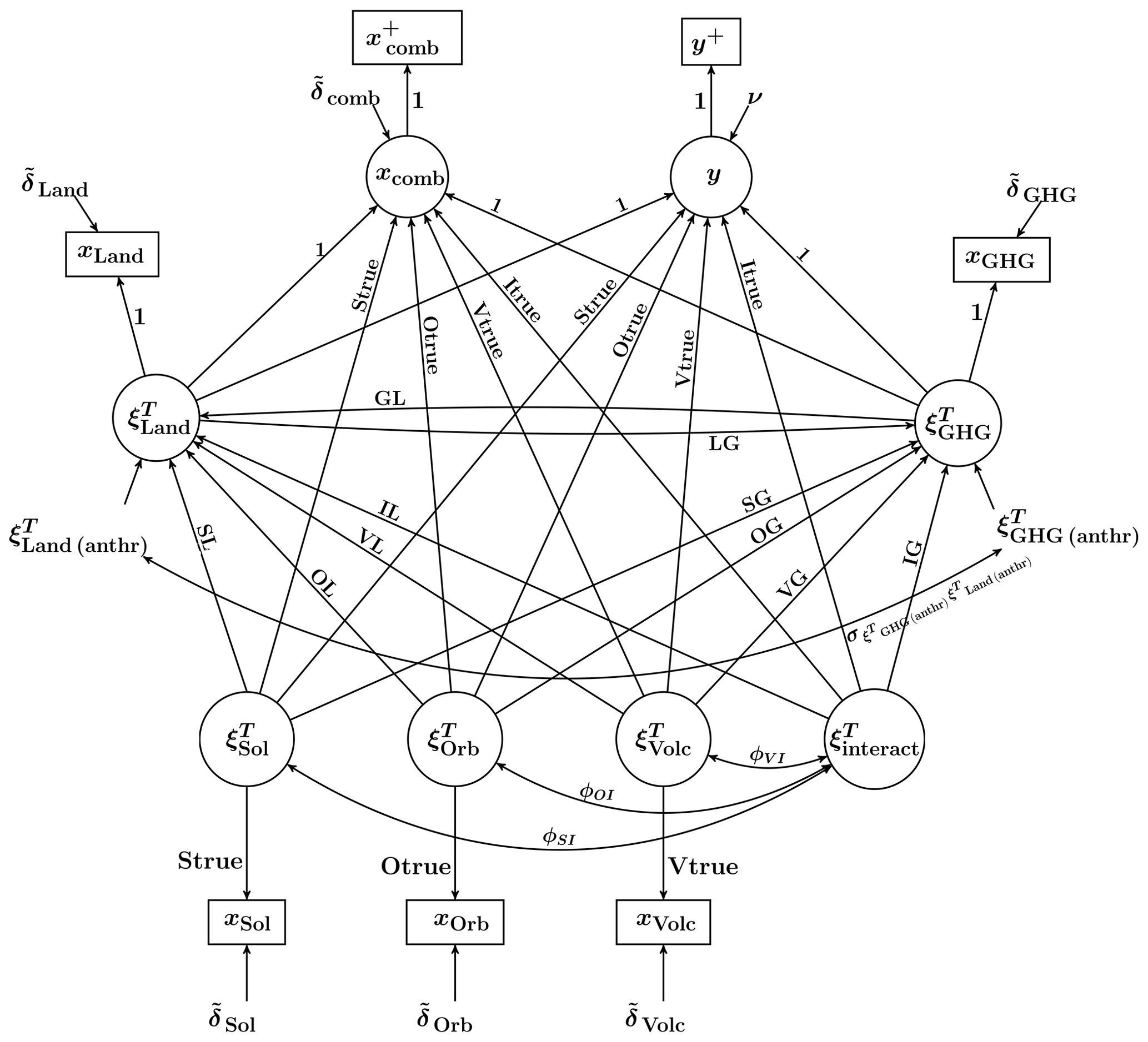
Figure 2Path diagram of a non-recursive (i.e. containing reciprocal relationships) SEM model under the hypothesis of consistency. The variance of each specific factor is assumed to be known a priori.
The important features of the SEM model in Fig. 2 are as follows:
-
The latent variables , , , and are still exogenous and standardised variables.
-
The latent variables and are endogenous variables. Since the variances of endogenous variables are not model parameters, and cannot be standardised. Instead, their coefficients in relation to their indicators are fixed to 1. Importantly, the variances of endogenous variables can be calculated afterwards (for details, see the Supplement), which makes it possible to compare the effect of the Land and GHG forcings on the temperature to the effect of other forcings under study. When relaxing the hypothesis of consistency in regard to and/or , one allows these latent factors to influence y with a magnitude equal to Ltrue and Gtrue, respectively, and, at the same time, keeps the magnitude of their impact on xcomb, xLand, and xGHG at 1.
-
The common factors , , and are still uncorrelated to each other. In addition, they are modelled as causally independent of and . This is because it is physically unjustified to assume that any changes in the Land and GHG forcing are capable of causing changes in the solar irradiance, the Earth's orbit, or the occurrence of volcanic eruptions.
-
There are two “new” observable variables, namely and y+. Neither of these two variables contains a disturbance term, implying that and . The difference is that xcomb and y are regarded as latent variables, while and y+ are regarded as observable. The introduction of the new variables allows us to satisfy the requirement of the SEM theory of disjoint sets of observable indicators for latent exogenous and for latent endogenous variables.
-
The anthropogenic components and are modelled as disturbance terms of and , respectively. Treating them as separate latent factors is not possible due to the assumption that only xLand and xGHG are available. For the same reason, they are related to each other through correlation. That is, they are modelled as if they were causally independent of each other, although it is climatologically motivated to assume their causal mutual dependence due to the common source that is human activity.
Just as the previously presented CFA models, the SEM model in Fig. 2 is a basic model, constituting a point of departure for constructing different SEM models. This can be accomplished either by deleting some of the depicted paths or by adding new ones. For example, in order to reflect the idea that the changing climate itself can cause subsequent changes, one can introduce causal paths from xcomb and/or y back to and/or or more precisely to and embedded in and , respectively. Note that these paths also express the idea that the internal processes can randomly contribute to natural changes in the Land and GHG forcings.
The same ideas can also be expressed by letting the observable x𝚏 variables impact and/or . From the perspective of structural equation modelling, freeing paths from observed variables to latent ones entails the movement from the general standard representation of a SEM model to its alternative representation (for details of both representations, see the Supplement). The identifiability status of each initial model should be determined on a case-by-case basis.
An initial SEM model, formulated on the basis of the basic SEM model, in accordance with climatological knowledge may also be modified empirically. Useful means in providing clues to specific model expansions are modification indices (for the details see Appendix A5). The main statistical advantage of model expansions is that they improve (to various extent) the overall model fit to data. Nevertheless, such modifications should be made judiciously as they lead to a reduction in the degrees of freedom. If an initial SEM model, on the other hand, demonstrates a reasonable fit both statistically and heuristically, model simplifications might be of more interest than model expansions.
In connection with empirical data-driven modifications of SEM (and CFA) models, we would also like to emphasise that the choice of a final or tentative model should not be made exclusively on a statistical basis – any modification ought to be defensible from the climatological point of view and reflect our knowledge about both the real-world climate system and the climate model under consideration. Also, a final SEM (and CFA) model should not be taken as a correct model, even if the model was not obtained as a result of empirical modifications. When accepting a final model, we can only say that “the model may be valid” because it does not contradict our assumptions and substantive knowledge.
In Sect. 4, we suggested estimators (14) and (15) for obtaining a priori estimates of the simulated internal temperature variability. Both estimators are associated with the following assumptions:
- i.
The variances of :s within an ensemble are equal.
- ii.
The sequences within an ensemble are mutually uncorrelated across all k𝚏 replicates.
- iii.
The magnitude of the forcing effect is the same for each ensemble member.
Each assumption is justified, both from the climate modelling perspective and statistically. However, if at least one of them is violated, the estimators may result in biased estimates. As a consequence, inferences about systematic influence of forcings on the temperature may be (seriously) flawed. In addition, it may deteriorate the overall fit of the previously presented CFA and SEM models to the data so they may be falsely rejected.
A possible way to check the validity of the estimators is to analyse the ensemble members by means of an appropriate CFA model. To this end, two simple CFA models were formulated. Their description is given in Sect. 6.1. In Sect. 6.2, we illustrate a practical application of one of these models, thereby demonstrating practical details of fitting a CFA model.
6.1 CFA models for analysing members of an ensemble
Using the definition of x𝚏 in Eq. (9), and without assuming that the forcing
f has a negligible effect on the temperature variability, the x𝚏 ensemble can be
analysed by the following CFA(k𝚏,1) model with a standardised latent factor:
where , , and is assumed to be uncorrelated with all . The CFA(k𝚏,1) model is associated with the same assumptions applied to estimator (14). Notice that since observational data are not involved, the specific factor includes only without involving (compare, for example, to Eq. 10).
Model (18) has two free parameters, α𝚏 and . They are estimable if at least two replicates are available. The more replicates, the more degrees of freedom the model χ2 test statistic, defined in Eq. (A5), has.
If the model fits the data adequately both statistically or heuristically, and the resulting estimate of α𝚏 is admissible and climatologically defensible, we may say that there is no reason to reject the associated assumptions. In that case, the whole ensemble is accepted for building the mean sequence, and the resulting estimate of is expected to be approximately the same as the estimate provided by estimator (14). Consequently, any of the two variance estimates can be used in the further analysis of the CFA and SEM models presented in the previous sections.
A corresponding CFA model associated with estimator (15) is obtained by imposing the restriction α𝚏=0 in the CFA(k𝚏,1) model (provided, of course, this restriction is climatologically justified). The resulting model has no latent factors; thus, it is called the CFA(k𝚏,0) model.
6.2 Numerical example
6.2.1 Data
We have analysed simulated near-surface temperatures generated with the Community Earth System Model (CESM) version 1.1 for the period 850–2005, the CESM-LME (Last Millennium Ensemble), which includes single-forcing ensembles with each of solar, volcanic, orbital, land, and GHG forcing alone, as well as several simulations where all forcings are used together. The CESM-LME experiment used 2∘ resolution in the atmosphere and land components and 1∘ resolution in the ocean and sea ice components. A detailed description of the model and the ensemble simulation experiment can be found in Otto-Bliesner et al. (2016) and references therein.
For the purpose of illustrating a practical application of a CFA model, we analyse xVolc ensembles for two regions, namely the region of the Arctic and Asia. The regions were defined as in PAGES 2k Consortium (2013) and also used by PAGES2k-PMIP3 group (2015). As seen in Fig. 1 in the former paper, the region of Arctic includes both land and sea surface temperatures, while Asia includes land-only temperatures. Each ensemble contains five replicates, each of which was forced only with a reconstruction of the transient evolution of volcanic aerosol loadings in the stratosphere, as a function of latitude, altitude, and month.
Annual-mean temperatures are used for the Arctic and the warm-season temperatures (JJA) for Asia. This choice depends on what was considered by the PAGES 2k Consortium (2013) as being the optimal calibration target for the climate proxy data they used. To extract seasonal temperature data from this simulation experiment such that they correspond to the regions defined in the PAGES 2k Consortium (2013) study, we followed exactly the same procedure as in the model vs. data comparison study undertaken by the PAGES2k-PMIP3 group (2015). After extraction, our raw temperature data sequences have a resolution of one temperature value per year, covering the 1000-year-long period 850–1849 AD. The industrial period after 1850 AD has been omitted in order to avoid a complication due to the fact that the CESM simulations for this last period include ozone–aerosol forcing, which is not available for the time before 1850. The plots of the raw data are given in Fig. S2 in the Supplement. The set of simulation temperature data sequences that we use here is a subset of the dataset published by Moberg and Hind (2019).
Two important aspects to remember when applying CFA and SEM models (as well as ME models) are that these models assume that data are normally distributed and do not exhibit autocorrelation. Since the forced component of simulated temperatures, i.e. , is treated as repeatable, the assumptions above concern the sequences, which, however, are not directly observable. Consequently, the series to check are
where denotes the average of k𝚏 replicates at time t.
Here, to avoid autocorrelation, all raw xVolc sequences were time-aggregated by taking 10-year non-overlapping averages. The same approach of avoiding autocorrelation was applied in SUN12. The resulting time series, each of which contains 100 observations of 10-year mean temperatures, are shown in Fig. S3 in the Supplement.
As supported by Fig. S4 in the Supplement, the assumption of time-independent observations is satisfied (because at least 91 % of the autocorrelation coefficients are insignificant as they are within the 90 % confidence bounds). Further, Fig. S4 in the Supplement also suggests that the decadally resolved residual sequences also demonstrate reasonable compliance with a normal distribution. This conclusion was also supported by the Shapiro–Wilk test (Shapiro and Wilk, 1965), whose results, however, are not shown.
6.2.2 Results
In the present work, we have used the R package sem
(see Fox et al., 2014, http://CRAN.R-project.org/package=sem, last access: 11 November 2022), which, in contrast to other broadly
used software designed to do CFA and SEM (e.g. LISREL, Mplus, Amos), is
an open-source alternative. The distinguishing feature of sem is that it requires
latent variable variances of 1 to be represented explicitly. In other words, latent variables and
coefficients in statistical models analysed are standardised.
The main steps of the estimation procedure in sem are described in
the Supplement by the example of our CFA model in Eq. (18).
The associated resulting outputs, produced by sem, are shown here
in Table 3, for the sake of convenience.
Table 3(A part of) Outputs produced by the R package sem as a result of fitting the CFA(5, 1) model from
Eq. (18) to two xVolc ensembles belonging to the region Asia and the Arctic, respectively.
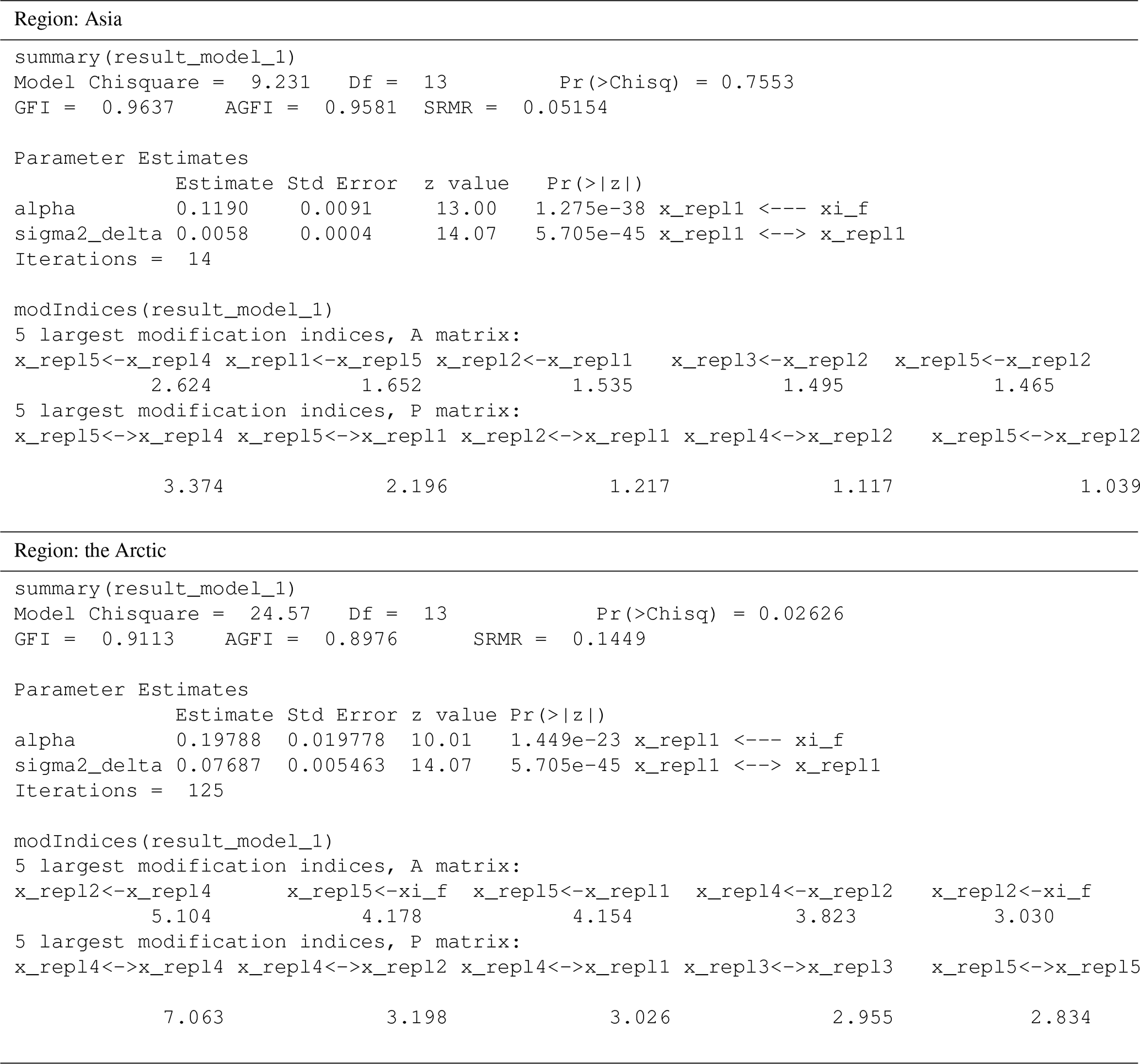
According to Table 3, the solution for the Asia data converged in 14 iterations, yielding an admissible (i.e. ) and climatologically reasonable solution. The latter follows from the fact that , equal to 0.1190 with a p value of less than 0.01, is statistically significant at all significance levels, which coincides with our expectations of a well-pronounced effect of the volcanic forcing, especially in the region of Asia.
Concerning the overall model fit, the output indicates that the model fits the data very well, both statistically and heuristically. Indeed, the model χ2 statistic of 9.23 with 13 degrees of freedom is associated with the p value of 0.75, which is far above the 5 % significance level. Further, the heuristic goodness-of-fit indices, GFI (goodness-of-fit index; see Eq. A6 in the Appendix) and AGFI (GFI adjusted for degrees of freedom; see Eq. A7 in the Appendix) (both equal to 0.96), are not only larger than the recommended cut-off limits of 0.90 and 0.80, respectively, but are also close to 1. A small SRMR value of 0.052, which is less than the recommended cut-off of 0.08, also indicates adequate fit to the data.
The output also contains information about the modification indices. The A matrix concerns
coefficients associated with different paths, while the P matrix contains information
about variances, covariances, and correlations. An entry in the A matrix is of the form
<endogenous variable>: <exogenous variable>;
i.e. the first variable is the variable the path goes to. Each of the variables can be either
latent or observable. Thus, when updating a CFA model to another CFA model, one is looking only
at paths from a latent variable to an observable variable. In the output associated with
the Asia data, none of the five suggested paths is such. Moreover, none of them suggest a substantial
reduction in the model χ2 statistic – the largest modification index of 2.62 is less than
the 5 % tabular value of χ2 with 1 degree of freedom, that is 3.84.
For the Arctic data, the conclusions are opposite. That is, the CFA(5, 1) model is rejected both statistically and heuristically. The model χ2 statistic of 24.57 with 13 degrees of freedom is associated with a p value of 0.026, which is less than 0.05. Probably, one could accept the model statistically at the 1 % significance level, but the heuristic indices, in particular the very high SRMR value (0.145>0.08), indicate an inadequate model fit to the data.
The same conclusion is indicated by the modification indices, suggesting that the model fit can be substantially improved.
The largest modification index of 7.063 (with 1 df) suggests that
the replicate number 4 differs from the other replicates in terms of the internal
variability. In addition, the largest modification index for the A matrix that is
applicable within the CFA specification (see the index equal to 4.178, labelled
x_repl5xi_f) also suggests that the replicate number 5 differs in terms of
the estimated magnitude of the simulated temperature response to the volcanic forcing.
We refrain from discussing possible reasons for the observed differences between the replicates and whether the reasons, suggested by the modification indices, are true or not. We can only say that if one wishes to continue the analysis of all ensembles by means of the CFA and/or SEM models suggested here, it is then motivating to try refitting the CFA(kVolc,1) model to a reduced xVolc ensemble, where kVolc equals either 4 or 3, depending on the number of replicates eliminated.
The present paper provides a theoretical background of a new statistical framework for the evaluation of simulated responses to climate forcings against observational climate data. A key idea of the framework, comprising two groups of statistical models, is that the process of evaluation should not be limited to a single statistical model. The models suggested here are CFA and SEM models, each of which is based on the concept of latent variables. Although they are closely related to each other, there are several differences between them, which allow for a statistical modelling of climatological relationships in various ways.
The idea of using CFA and SEM models originates from D&A fingerprinting studies employing statistical models known as measurement error (ME) models (or equivalently errors-in-variables models). As a matter of fact, an ME model is a special case of a CFA model, which means that an ME model is a special case of a SEM model as well. In the present work, using this close connection between the three types of statistical models, the ME model specification has been extended first to the CFA and SEM model specifications.
The theoretical results of this work have demonstrated that both CFA and SEM models, just as ME models in D&A studies, are, first of all, capable of addressing the questions posed in D&A studies, namely the assessment of the contribution of the forcings to the temperature variability (the questions of detection and attribution) and the evaluation of climate model simulations in terms of temperature responses to forcings (the question of consistency). In addition, the extensions have provided the following advantageous possibilities:
-
The structure of the underlying relationships can be varied between latent temperature responses to forcings in accordance to their properties and interpretations. For example, one may assume that latent temperature responses to some forcings among those considered are mutually uncorrelated. Such restrictions are especially desirable for analysing climate data associated with the so-called weak-signal regime.
-
The assumption of the additivity of forcing effects can be relaxed. At this point, let us remark that according to Bollen (1989, p. 405), it does not seem completely impossible to incorporate term(s) representing the effect of various interactions within ME models. But the methods suggested are definitely more complicated than to fit a CFA model, and, what is more important, they do not allow for the evaluation of multi-forcing climate model simulations.
-
Multi-forcing climate model simulations can be evaluated not only in terms of the overall forcing effect to a combination of forcings (see Sect. 1.2 in the Supplement), but also in terms of individual forcing effects.
-
Non-climatic noise in observational data can be taken into account.
-
The contribution of each forcing to the observed temperature variability can be assessed and the simulated responses to climate forcings evaluated, not only simultaneously but also separately if needed.
-
Complicated climatological feedback mechanisms within the SEM model specification can be statistically modelled, which allows for various causal relationships not permitted within either ME or CFA models.
It can also be noted that the application of SEM in general is possible under a wide range of distributional assumptions; see, for example, Finney and DiStefano (2006), or Bollen (1989, pp. 415–445). In the framework presented, the climate variable of interest is temperature, assumed to have a normal distribution. However, the ideas of the framework may pave the way for future studies focusing on other climate variables, for example, precipitation or drought/wetness indices, that may require other distributional assumptions and other estimation methods than likelihood estimation.
Here, we would like to point out that the underlying latent causal structures suggested in this work are only rough approximations of the real-world climatological feedback mechanisms. The degree of approximation depends directly on the availability of climate model simulations driven by various combinations of the forcings of interest. In the present work, it was assumed that only one type of multi-forcing simulations is available, namely a simulation generated by a climate model driven by all forcings of interest simultaneously. As a result, the departure from the additivity of individual forcing effects could be modelled only by a single latent variable, which represented an overall effect of possible interactions of the forcings of interest, regardless of their origin. The impossibility to split this interaction term into several subcomponents, each of which is either of natural or anthropogenic character, entails certain interpretation difficulties of some relationships within our SEM model. However, the issue can be resolved as soon as more multi-forcing simulations, driven by various combinations of forcings, are available. The issue also becomes irrelevant under the assumption of additivity.
Other limitations of the presented statistical models presented here are as follows:
-
They are formulated under the assumption of no autocorrelation, which is unrealistic in the case of climate data. To overcome this issue, it was suggested here to perform a time aggregation of the data (both simulated and real-world), which unavoidably reduces the sample size. Depending on the period of interest, the reduction may be substantial, which may lead to unreliable statistical inferences. In such situations, to accept larger sample sizes, however, would mean that one has to accept a certain autocorrelation. Thus, in future work, it is of interest to investigate the impact of various levels of autocorrelation on the validity of significance tests. Another research question of interest concerns other ways of compensating for the presence of autocorrelation, for example, by replacing the sample size by the effective sample size (Faes et al., 2009).
-
They are formulated under the assumption of a time-constant variance of observational data. This assumption is likely to be violated when data cover both pre-industrial and industrial periods. Some research on this topic has already been done (Fetisova, 2015, Sect. 2.4). However, it may be of interest to investigate other possible methods of taking time-varying variances into account.
-
They are suitable for analysing data from a single region only. That is, they do not allow for a simultaneous assessment of a given forcing's contribution within each region under consideration. To be able to perform such multi-regional analyses, meaning that the resulting variance–covariance matrix of observed variables comprises several regional variance–covariance matrices in a block manner, the CFA (and SEM) models need to be extended accordingly. Conceivable starting points for this work can be found in Fuller (1987, pp. 325–327) and Wall (2012).
-
The methods presented here do not involve dimensionality reduction (including pre-whitening), which is performed in D&A studies (Allen and Stott, 2003; Gillett et al., 2004a; Shiogama et al., 2016; Tett et al., 1999). The main reason for not addressing this issue here is our wish to avoid excessive complexity in a first work describing a new framework. However, keeping in mind the close statistical relations between the ME, CFA, and SEM models, we see no obvious obstacles (at least, theoretically) to applying the method of dimensionality reduction (including pre-whitening), used in D&A studies, to the models within our framework. This issue can certainly be investigated in depth in future research. The range of research questions may include both those that are pertinent to D&A studies, such as the issues of estimating the pre-whitening matrix (Ribes et al., 2013) and the impact of using an estimate of this matrix on the coverage rate of the confidence intervals (Li et al., 2021), and the questions motivated by our framework, for example, possible modifications of our CFA and SEM models in order to take into account the difference in the interpretations of unforced variability (compare (νg, ) in Eq. 1 to (δt, νt)′, defined in Eqs. 10 and 8, respectively).
-
In practice, fitting large over-identified CFA and SEM models (with many observable variables) is expected to be challenging, both from the statistical and climatological perspective, compared to ME models used in D&A studies, which ultimately may require close collaboration between statisticians, paleoclimatologists, and climate modellers.
Despite the above-mentioned limitations of our framework, we firmly believe that the framework has a capacity to become a powerful and flexible tool for deriving valuable insights into the properties of climate models and the role of climate forcings in climate change, which ultimately may improve our understanding of various mechanisms and processes in the real-world climate system. Moreover, its degree of flexibility in forming an appropriate statistical model can further be increased by viewing the ME model specification as a part of the framework. According to the principle of parsimony, it is always motivating to prefer a simpler model demonstrating an acceptable and adequate performance to a more complicated one.
Our concluding remark is that the characteristics of the statistical models within our framework, capable of addressing the questions posed in D&A studies, were discussed only theoretically. Prior to employing them in practical analyses involving real-world observational data, their performance needs to be evaluated in a controlled numerical experiment, within which it is known that the simulated temperature responses to forcings of interest are correctly represented, both in terms of their magnitude and shape. This will be the purpose of the analysis presented by Lashgari et al. (2022).
A1 The definition of a CFA model
A general CFA model with q observed mean-centred variables and p latent common factors,
in which xt is a q×1 vector of observed variables at time point t, ξt is a p×1 vector of latent common factors that are assumed to be responsible for the correlation among the observed variables, Λ is a q×p matrix of coefficients connecting ξt to xt, and δt is a q×1 vector of errors.
In the terminology of factor analysis, the observed variables are called indicators or manifest variables. The coefficients Λ are referred to as factor loadings. The δt variables are often called specific factors because they are specific to the particular indicator they are associated with. They are assumed to be identically and independently distributed, more precisely N(0,diagΣδ). In addition, they are assumed to be uncorrelated with ξt, which in turn can be treated either as random (typically normally distributed with zero mean) or as a fixed unknown constant. In contrast to the specific-factor variables, common factors can be either correlated or uncorrelated with each other.
The main characteristic of CFA is that the researcher formulates a factor model, or a set of models, in accordance with a substantive theory about the underlying common factor structure. That is, the number of latent factors, their interpretation, and the nature of the factor loadings are specified a priori. In addition, researchers can have certain hypotheses, which results in additional restrictions on the parameter space. A typical classification of parameters within CFA is the following (Jöreskog, 1969, 1976):
-
A free parameter is a parameter to be estimated. Since free parameters are not associated with anything specific about them, they are not a part of the hypotheses associated with a factor model.
-
A fixed parameter is a parameter whose value is prespecified by hypothesis, and this value remains unchanged during the iterative estimation process.
-
A constrained-equal parameter is a parameter that is estimated, but its value is constrained to be equal to another parameter (or parameters). Because only one value needs to be determined for each group of constrained-equal parameters, only one parameter from this group is counted when counting the number of distinct estimated parameters. In contrast to free parameters, constrained-equal parameters are a part of the hypotheses associated with a factor model, although both types of parameters are estimated.
A2 Estimation of the parameters
The estimation of parameters in CFA is based on the idea that the population variance–covariance matrix of the indicators, Σ, can be represented as a function of the model parameters θ, denoted Σ(θ). The matrix Σ(θ) is called the implied (or model's reproduced) variance–covariance matrix of the indicators. The objective of CFA is to empirically confirm or disconfirm the hypothesised latent structure or equivalently the hypothesised variance–covariance matrix of the indicators. Thus, the parameters are estimated such that the discrepancy between the sample variance–covariance matrix of the indicators, S, and the estimated model's reproduced variance–covariance matrix, , is as small as possible. In particular, under the assumption of normality of the data, the estimates are obtained by minimising the following discrepancy function with respect to the free parameters, conditional on the explicitly constrained parameters (Bollen, 1989; Jöreskog, 1969; Mulaik, 2010):
As shown by Jöreskog (1969), minimising Eq. (A2) is equivalent to maximising the maximum likelihood (ML) function, which implies that the estimates obtained are ML estimates. According to the general theory, the ML estimates are consistent, jointly asymptotically normally distributed with the asymptotic variance expressed as being the inverse of the Fisher information. In CFA, the Fisher information matrix is defined as follows:
The inverse of Eq. (A3), evaluated at the values for the parameters that minimise the F function, gives an estimate of the variance of the asymptotic distribution of the model estimates.
One can use the estimated variances to test each estimated parameter θi by means of the z statistic , which has approximately a standard normal distribution. The results of tests that θi=0 are provided in the form of two-sided p values by all statistical packages designed to do CFA, regardless of whether a model is just-identified or over-identified. In addition, one also can construct the approximate 100(1−p)% Wald confidence interval for each parameter θi to test :
where is the percentile of the standard normal distribution.
A3 The concept of identifiability
A key concept in CFA is identifiability of parameters. Identifiability is closely related to the ability to estimate the model parameters from a sample generated by the model, given restrictions imposed on the parameters. The general identifiability rule states that if an unknown parameter θi can be written as a function of one or more elements of Σ, that parameter is identified (see Bollen, 1989, p. 89). If all unknown parameters in θ are identified, then the model is identified.
Based on this definition of identifiability, a factor model can be classified as under-identified, just-identified, or over-identified. Obviously, free parameters cannot be estimated from any Σ if their number exceeds the number of the non-duplicated (unique) elements in Σ equal to . Therefore, such a factor model is called under-identified. Just-identified models have as many parameters as the number of the unique equations in Σ, and, most importantly, each parameter can be explicitly solved in terms of the variances and covariances of the indicators.
For over-identified models, the number of free parameters is smaller than the number of unique equations σij=σij(θ), and more than one distinct equation is solvable for (some) θi. As a consequence, over-identified parameters have multiple solutions, implying that the minimisation of the discrepancy function in question is performed numerically. This entails that S does not fit perfectly, thus making it meaningful to assess the fit of the model to the data. For just-identified models, assessing the overall fit and hypothesis testing are senseless because of the fact that Σ(θ)=S is a mathematical necessity, not an empirical finding.
Notice that even if the number of free parameters is smaller than or equal to the number of unique equations in Σ=Σ(θ), but at least one free parameter cannot be written as a function of the elements of Σ, the associated factor model is clearly under-identified.
One way to establish the identifiability is to solve structural covariance equations Σ=Σ(θ) for unknown parameters in θ algebraically. However, for large models with many indicators, the attempts of establishing their identifiability algebraically are very likely to be error-prone and time-consuming. Given such a situation, researchers may resort to empirical tests for identifiability.
One of them is the empirical test of the matrix of second-order derivatives of the discrepancy function in Eq. (A2) used to estimate the model. According to Jöreskog and Sörbom (1989), “if the model is identified, the information matrix is almost certainly positive definite. If the information matrix is singular, the model is under-identified”. The test is automatically calculated in all statistical packages developed to estimate structural equation models, for example, LISREL, EQS, and the R package sem.
According to Jöreskog and Sörbom (1989), identifiability can also be checked by the following two-step test. The first step is to analyse the sample variance–covariance matrix, S, as usual and to save the predicted covariance matrix based on the estimates of the model parameters, i.e. . Next, substitute for S, and rerun the same program. If the model is identified, the new estimates should be identical to the first ones that were generated.
Yet another possible check for identifiability is to estimate the model with different starting values for free parameters in the iterative estimation algorithm to see whether or not the algorithm converges to the same parameter estimates each time. This empirical test, however, should be used with great care. Choosing inappropriate starting values may cause the failure of convergence, although the model is theoretically identified.
In practice, the estimation procedure may produce parameter estimates, although the model is theoretically under-identified. Such a phenomenon is known as empirical under-identifiability (Rindskopf, 1984), causing inadmissible solutions. One way to check whether a solution is admissible or not is to look at the completely standardised solution. This type of solution standardises the solution such that the variances of the latent factors and the indicators are 1. Inadmissible solutions are indicated by factor loadings and correlation coefficients exceeding 1 and by specific-factor variances that are negative or are greater than 1. Inadmissible estimates of correlation coefficients can also be detected by means of the standardised solution, associated with a CFA model, where only latent factors are standardised to have their variances equal to 1.
In order to avoid empirical under-identifiability, and in order to undertake justified empirical modifications of the model in case they are needed, it is important to identify the causes of the model's theoretical under-identification prior to estimating a CFA model. To this end, it would be sufficient to ensure that each parameter is solvable from structural covariance equations, without deriving closed analytical expressions of the solution.
Examining the variance–covariance matrix of the asymptotic distribution of the model estimates is also helpful for revealing empirical under-identifiability. If the model is nearly under-identified, it will be reflected in high covariances between two or more parameter estimates.
Even if estimates are admissible, one should also ensure that they have the anticipated signs and magnitudes.
A4 Assessing the overall model fit
For just-identified CFA models, the function , evaluated at the minimum, is equal to zero, since and . That is, a just-identified model has an exact solution in terms of the variances and covariances among indicators, but nothing is hypothesised, and nothing can be tested.
For over-identified models, arising due to additional constraints imposed on some model parameters, at least one (free) parameter can be expressed by more than one distinct equation in terms of the variances and covariances of indicators. Therefore, the fit between and the sample variance–covariance matrix, in general, will not be perfect, thus motivating assessment of the model fit to the data.
To this end, one uses the fact that the discrepancy function (A2) is related to the log-likelihood ratio χ2 goodness-of-fit test of the model's Σ(θ) to S (Jöreskog, 1969). The relation is given by
where is the logarithm of the likelihood function under the null hypothesis , while is the logarithm of the likelihood function under the alternative hypothesis HA of unrestricted Σ, i.e. Σ=S.
In large samples, the χ2 test statistic is approximately distributed as χ2 with degrees of freedom, where is the number of the unique (non-duplicated) equations in the variance–covariance matrix of the indicators, and m is the number of distinct free parameters.
If the solution obtained is admissible and interpretable, the statistical assessment of the overall model fit is performed by means of the χ2 test statistic. Note that failure to reject the null hypothesis is desired, as it leads to the conclusion that the hypothesised model is consistent with the data.
When applying the χ2 test statistic, it should be kept in mind that in large samples even small differences between S and can be statistically significant, although the differences may not be practically meaningful. Consequently, a number of goodness-of-fit indices, serving as heuristic measures of model fit, have been proposed in the factor analysis literature (see, for example, Hu and Bentler, 1998; Mulaik, 2010; Sharma, 1996). Some of them are as follows: a goodness-of-fit index (GFI), GFI adjusted for degrees of freedom (AGFI), and standardised root-mean-square residual (SRMR). Their definitions are the following (Hu and Bentler, 1999; Sharma, 1996):
where df is the degrees of freedom, q is the number of indicators, and
where sij:= observed (co)variances, reproduced (co)variances, and sii and sjj:= observed standard deviations.
As for cut-off values of the indices, the following rules of thumb have been recommended. The GFI for good-fitting models should be greater than 0.90, while for the AGFI the suggested cut-off value is 0.8 (Sharma, 1996). For the SRMR, a perfect model fit is indicated by SRMR =0. Consequently, the larger the SRMR, the less fit between the model and the data. According to Hu and Bentler (1999), a cut-off value close to 0.08 for SRMR indicates a good fit.
Notice that the goodness-of-fit indices can be used both for assessing the fit of a single CFA model and for a number of competing models fitted to the same data set.
A5 Empirical data-driven modifications of CFA models
According to the “pure” confirmatory approach, the rejection of the hypothesised model, whose estimated parameters are judged to be admissible and interpretable, means that one rejects the model and the associated underlying hypotheses, without proceeding with any updating of this hypothesised structure. However, in practice, researchers do proceed. The first aspect to check is whether no key elements of the underlying hypotheses are missing. Further, this motivates a check of other possible reasons of the poor model fit, such as small sample size, non-normality, or missing data (Boomsma, 2000). Finally, a typical approach to arriving at a CFA model with an adequate fit is to free some constrained parameters with the aid of modification indices.
Developed by Sörbom (1989), modification indices attempt to estimate which missing parameter, if added to the current CFA model, would result in the greatest reduction of the discrepancy between model and data. The way to use these indices is to free the fixed parameter associated with the largest reduction and reanalyse the resulting model. Hence, modification indices help us to establish the identifiability of modified models. If a modification index for a fixed parameter is not zero and positive, this indicates that this parameter will be identified if it is set free.
Modified models suggested by modification indices are so-called nested models, fitted to the same data. That is, each of them is a special case of the initial model, where the parameter suggested to be estimated, is constrained to zero. According to statistical theory in Steiger et al. (1985), for nested models, one can treat the difference in the two χ2 values as a χ2 difference statistic with degrees of freedom equal to the difference in their degrees of freedom.
The present work employed the R package sem
(Fox et al., 2014; Fox, 2006) (http://CRAN.R-project.org/package=sem, https://doi.org/10.1207/s15328007sem1303_7) using R version 3.0.2 (R Core Team, 2013) (http://www.R-project.org/, last access: 6 December 2022).
The R package sem was used for the estimation of the CFA(k𝚏, 1) model,
given in Eq. (18). The R code is given in the Supplement to
this article (see Sect. S4). The simulation data used in this study are available from the Bolin Centre Database, Stockholm University (Moberg and Hind, 2019, https://doi.org/10.17043/moberg-2019-cesm-1). The data are the same as used in Fetisova (2017) (http://su.diva-portal.org/smash/record.jsf?pid=diva2:1150197&dswid=9303, last access: 6 December 2022).
The supplement related to this article is available online at: https://doi.org/10.5194/ascmo-8-225-2022-supplement.
This work is based on ideas presented in a doctoral thesis in mathematical statistics by Ekaterina Fetisova (Fetisova, 2017), who later changed her name to Katarina Lashgari (KL). The doctoral thesis work was carried out from 2013 to 2017. At that time, the co-authors GB, AM, and RS were involved as supervisors. Afterwards, KL led the further development of the methodology and introduced the idea of employing SEM, and she is the lead author of this paper. GB contributed partly to the development of the methodology, commented on the manuscript text, and helped write some of it. AM introduced, in an early stage of the work on the doctoral thesis, the idea to study the relationship between the statistical method used in many D&A studies and the method used by Sundberg et al. (2012). He also contributed to the discussion from the perspective of climate science and helped write some of the text. RS proposed, in an early stage of the work, to study the role of just-identified CFA models in this context and contributed to their development. In a late stage, he also contributed with comments to the manuscript underlying this paper.
The contact author has declared that none of the authors has any competing interests.
Publisher's note: Copernicus Publications remains neutral with regard to jurisdictional claims in published maps and institutional affiliations.
The authors would like to thank Qiong Zhang (Department of Physical Geography, Stockholm University) for helpful explanations of some aspects of climate modelling.
This research was funded by the Swedish Research Council (grant C0592401 to Gudrun Brattström, ”A statistical framework for comparing paleoclimate data and climate model simulations”).
This paper was edited by Francis Zwiers and reviewed by two anonymous referees.
Allen, M. R. and Stott, P. A.: Estimating signal amplitudes in optimal fingerprinting, part I: theory, Clim. Dynam., 21, 477–491, https://doi.org/10.1007/s00382-003-0313-9, 2003. a, b, c, d, e
Bollen, K. A.: Structural equations with latent variables, Wiley, ISBN 0471011711, 1989. a, b, c, d
Boomsma, A.: Reporting Analyses of Covariance Structures, Struct. Equ. Modeling, 7, 461–483, https://doi.org/10.1207/S15328007SEM0703_6, 2000. a
Brohan, P., Kennedy, J. J., Harris, I., Tett, S. F. B., and Jones, P. D.: Uncertainty estimates in regional and global observed temperature changes: A new data set from 1850, J. Geophys. Res., 111, D12106, https://doi.org/10.1029/2005JD006548, 2006. a
Cheng, C.-L. and van Ness, J. W.: Statistical regression with measurement error, Kendall's Library of Statistics, Oxford University Press Inc., New York, ISBN 0340614617, 1999. a
Cubasch, U., Wuebbles, D., Chen, D., Facchini, M. C., Frame, D., Mahowald, N., and Winther, J.-G.: Introduction, in: Climate Change 2013: The Physical Science Basis. Contribution of Working Group I to the Fifth Assessment Report of the Intergovernmental Panel on Climate Change, edited by: Stocker, T. F., Qin, D., Plattner, G.-K., Tignor, M., Allen, S. K., Boschung, J., Nauels, A., Xia, Y., Bex, V., and Midgley, P. M., Cambridge University Press, Cambridge, United Kingdom and New York, NY, USA, 2013. a
DelSole, T., Trenary, L., Yan, X., and Tippett, M. K.: Confidence intervals in optimal fingerprinting. Clim. Dynam., 52, 4111–4126, https://doi.org/10.1007/s00382-018-4356-3, 2019. a, b
Deser, C., Phillips, A., Bourdette, V., and Teng, H.: Uncertainty in climate change projections: the role of internal variability, Clim. Dyna,, 38, 527–546, https://doi.org/10.1007/s00382-010-0977-x, 2012. a
Eyring, V., Bony, S., Meehl, G. A., Senior, C. A., Stevens, B., Stouffer, R. J., and Taylor, K. E.: Overview of the Coupled Model Intercomparison Project Phase 6 (CMIP6) experimental design and organization, Geosci. Model Dev., 9, 1937–1958, https://doi.org/10.5194/gmd-9-1937-2016, 2016. a
Faes, C., Molenberghs, G., Aerts, M., Verbeke, G., and Kenward, M. K.: The effective sample size and analternative small-sample degrees-of-freedom method, Am. Stat., 63, 389–399, https://doi.org/10.1198/tast.2009.08196, 2009. a
Fetisova, E.: Evaluation of climate model simulations by means of statistical methods, licentiate thesis, http://www.math.su.se/polopoly_fs/1.260101.1449662582!/menu/standard/file/LicUppsats_KatarinaF.pdf (last access: 11 November 2022), 2015. a, b
Fetisova, E.: Towards a flexible statistical modelling by latent factors for evaluation of simulated climate forcing effects, doctoral thesis, Department of Mathematics, Stockholm University, http://su.diva-portal.org/smash/record.jsf?pid=diva2%3A1150197&dswid=9303 (last access: 11 November 2022), 2017. a, b
Feulner, G.: Are the most recent estimates for Maunder Minimum solar irradiance in agreement with temperature reconstructions?, Geophys. Res. Lett., 38, L16706, https://doi.org/10.1029/2011GL048529, 2011. a
Finney, S. J., and DiStefano, C.: Non-normal and categorical data in structural equation modeling in: Structural equation modeling: A second course, edited by: Hancock, G. R. and Mueller, R. O., Greenwich, Connecticut: Information Age Publishing, 269–314, 2006. a
Flato, G., Marotzke, J., Abiodun, B., Braconnot, P., Chou, S. C., Collins, W., Cox, P., Driouech, F., Emori, S., Eyring, V., Forest, C., Gleckler, P., Guilyardi, E., Jakob, C., Kattsov, V., Reason, C., and Rummukainen, M.: Evaluation of Climate Models, in: Climate Change 2013: The Physical Science Basis. Contribution of Working Group I to the Fifth Assessment Report of the Intergovermental Panel on Climate Change, edited by: Stocker, T. F., Qin, D., Plattner, G.-K., Tignor, M., Allen, S. K., Boschung, J., Nauels, A., Xia, Y., Bex, V., and Midgley, P. M., Cambridge University Press, Cambridge, United Kingdom and New York, NY, USA, https://doi.org/10.1017/CBO9781107415324.020, 2013. a
Fox, J.: TEACHER'S CORNER: Structural Equation Modeling With the sem Package in R, Struct. Equ. Modeling, 13, 465–486, https://doi.org/10.1207/s15328007sem1303_7, 2006. a
Fox, J., Nie, Z., Byrnes, J., Culbertson, M., DebRoy, S., Friendly, M., Goodrich, B., Jones, R. H., Kramer, A., Monette, G., and R-Core: sem: Structural Equation Models, R package version 3.1-5, http://CRAN.R-project.org/package=sem (last access: 11 November 2022), 2014. a, b
Fuller, W. A.: Measurement Error Models, Wiley, ISBN 0-471-86187-1, 1987. a, b
Gettelman, A., and Sherwood, S.C.: Processes Responsible for Cloud Feedback. Current Climate Change Reports 2, 179–189, https://doi.org/10.1007/s40641-016-0052-8, 2016. a
Gillett, N. P., Weaver, A. J., Zwiers, F. W., and Flannigan, M. D.: Detecting the effect of climate change on Canadian forest fires, Geophys. Res. Lett., 31, L18211, https://doi.org/10.1029/2004GL020876, 2004a. a
Gillett, N. P., Wehner, M. F., Tett, S. F., and Weaver, A. J.: Testing the linearity of the response to combined greenhouse gas and sulfate aerosol forcing, Geophys. Res. Lett., 31, L14201, https://doi.org/10.1029/2004GL020111, 2004b. a
Goosse, H.: Climate system dynamics and modelling, Cambridge university press, USA, ISBN 9781107445833, 2015. a
Hasselmann, K.: On the signal-to-noise problem in atmospheric response studies, edited by: Shaw, D. B., Royal Meteorological Society, 251–259, 1979. a
Hasselmann, K.: Optimal Fingerprints for the detection of time-dependent climate change, J. Climate, 6, 1957–1971, https://doi.org/10.1175/1520-0442(1993)006<1957:OFFTDO>2.0.CO;2, 1993. a
Hasselmann, K.: Multi-pattern fingerprint method for detection and attribution of climate change, Clim. Dynam., 13, 601–611, https://doi.org/10.1007/s003820050185, 1997. a
Hegerl, G. C. and Zwiers, F.: Use of models in detection and attribution of climate change, Adv. Rev., 2, 570–591, https://doi.org/10.1002/wcc.121, 2011. a, b
Hegerl, G. C., Zwiers, F. W., Braconnot, P., Gillett, N. P., Luo, Y., Marengo Orsini, J. A., Nicholls, N., Penner, J. E., and Stott, P. A.: Understanding and Attributing Climate Change, in: Climate Change 2007: The Physical Science Basis, Contribution of Working Group I to the Fourth Assessment Report of the Intergovermental Panel on Climate Change, edited by: Solomon, S., Qin, D., Manning, M., Chen, Z., Marquis, M., Averyt, K. B., Tignor, M., and Miller, H. L., Cambridge University Press, Cambridge, United Kingdom and New York, NY, USA, 2007. a, b, c, d
Hegerl, G. C., Hoegh-Guldberg, O., Casassa, G., Hoerling, M. P., Kovats, R. S., Parmesan, C., Pierce, D. W., and Stott, P. A.: Good Practice Guidance Paper on Detection and Attribution Related to Anthropogenic Climate Change, in: Meeting Report of the Intergovernmental Panel on Climate Change Expert Meeting on Detection and Attribution of Anthropogenic Climate Change, edited by: Stocker, T. F., Field, C. B., Qin, D., Barros, V., Plattner, G.-K., Tignor, M., Midgley, P. M., and Ebi, K. L., IPCC Working Group I Technical Support Unit, University of Bern, Bern, Switzerland, 2010. a
Hegerl, G. C., Luterbacher J., Gonźalez-Rouco, F., Tett, S. F. B., Crowley, T., and Xoplaki, E.: Influence of human and natural forcing on European seasonal temperatures, Nat. Geosci., 4, 99–103, https://doi.org/10.1038/NGEO1057, 2011. a
Hind, A. and Moberg, A.: Past millennial solar forcing magnitude. A statistical hemispheric-scale climate model versus proxy data comparison, Clim. Dynam., 41, 2527–2537, https://doi.org/10.1007/s00382-012-1526-6, 2013. a
Hind, A., Moberg, A., and Sundberg, R.: Statistical framework for evaluation of climate model simulations by use of climate proxy data from the last millennium – Part 2: A pseudo-proxy study addressing the amplitude of solar forcing, Clim. Past, 8, 1355–1365, https://doi.org/10.5194/cp-8-1355-2012, 2012. a
Hu, L. and Bentler, P. M.: Fit indices in covariance structure modeling: sensitivity to underparameterized model misspecification, Psychol. Meth., 3, 424–453, https://doi.org/10.1037/1082-989X.3.4.424, 1998. a
Hu, L. and Bentler, P. M.: Cutoff criteria for fit indexes in covariance structure analysis: Conventional criteria versus new alternatives, Struct. Eq. Modeling, 6, 1–55, https://doi.org/10.1080/10705519909540118, 1999. a, b
Huntingford, C., Stott, P. A., Allen, M. R., and Lambert, F. H.: Incorporating model uncertainty into attribution of observed temperature change, Geophys. Res. Lett., 33, L05710, https://doi.org/10.1029/2005GL024831, 2006. a
Jones, P. D., Briffa, K. R., Osborn, T. J., Lough, J. M., van Ommen, T. D., Vinther, B. M., Luterbacher, J., Wahl, E. R., Zwiers, F. W., Mann, M. E., Schmidt, G. A., Ammann, C. M., Buckley, B. M., Cobb, K. M., Esper, J., Goosse, H., Graham, N., Jansen, E., Kiefer, T., Kull, C., Küttel, M., Mosley-Thompson, E., Overpeck, J. T., Riedwyl, N., Schulz, M., Tudhope, A. W., Villalba, R., Wanner, H., Wolff, E., and Xoplaki, E.: High-resolution palaeoclimatology of the last millennium: a review of current status and future prospects, Holocene, 19, 3–49, https://doi.org/10.1177/0959683608098952, 2009. a
Jungclaus, J. H., Bard, E., Baroni, M., Braconnot, P., Cao, J., Chini, L. P., Egorova, T., Evans, M., González-Rouco, J. F., Goosse, H., Hurtt, G. C., Joos, F., Kaplan, J. O., Khodri, M., Klein Goldewijk, K., Krivova, N., LeGrande, A. N., Lorenz, S. J., Luterbacher, J., Man, W., Maycock, A. C., Meinshausen, M., Moberg, A., Muscheler, R., Nehrbass-Ahles, C., Otto-Bliesner, B. I., Phipps, S. J., Pongratz, J., Rozanov, E., Schmidt, G. A., Schmidt, H., Schmutz, W., Schurer, A., Shapiro, A. I., Sigl, M., Smerdon, J. E., Solanki, S. K., Timmreck, C., Toohey, M., Usoskin, I. G., Wagner, S., Wu, C.-J., Yeo, K. L., Zanchettin, D., Zhang, Q., and Zorita, E.: The PMIP4 contribution to CMIP6 – Part 3: The last millennium, scientific objective, and experimental design for the PMIP4 past1000 simulations, Geosci. Model Dev., 10, 4005–4033, https://doi.org/10.5194/gmd-10-4005-2017, 2017. a, b, c, d
Jöreskog, K. G.: A general approach to confirmatory maximum likelihood factor analysis, Psychometrika, 34, 183–202, https://doi.org/10.1007/BF02289343, 1969. a, b, c, d
Jöreskog, K. G.: Structural equation models in the social sciences: specification, estimation and testing, Research rapport 16, University of Uppsala, Departments of Statistics, 33 pp., 1976. a
Jöreskog, K. G. and Sörbom, D.: LISREL 7: a guide to the program and applications, Chicago, III, SPSS INC, 1989. a, b, c
Kodra, A., Chatterjee, S., and Ganguly, A. R.: Exploring Granger causality between global average observed time series of carbon dioxide and temperature, Theor. Appl. Climatol., 104, 325–335, https://doi.org/10.1007/s00704-010-0342-3, 2011. a
Kutzbach, J. E.: The nature of climate and climatic variations, QuaternaryRes., 6, 471–480, https://doi.org/10.1016/0033-5894(76)90020-X, 1976. a
Lashgari, K., Moberg, A., and Brattström, G.: Evaluation of simulated responses to climate forcings: a flexible statistical framework using confirmatory factor analysis and structural equation modelling – Part 2: Numerical experiment, Adv. Stat. Clim. Meteorol. Oceanogr., 8, 249–271, https://doi.org/10.5194/ascmo-8-249-2022, 2022. a
Levine, R. A. and Berliner, L. M.: Statistical principles for climate change studies, J. Climate, 12, 564–574, https://doi.org/10.1175/1520-0442(1999)012<0564:SPFCCS>2.0.CO;2, 1999. a
Li, Y., Chen, K., Yan, J., and Zhang, X.: Uncertainty in optimal fingerprinting is underestimated, Environ. Res. Lett., 8, 084043. https://doi.org/10.1088/1748-9326/ac14ee, 2021. a
Liang, X. S.: Unraveling the cause-effect relation between time series, Phys. Rev. E, 90, 052150, https://doi.org/10.1103/PhysRevE.90.052150, 2014. a
Liepert, B. G.: The physical concept of climate forcing, WIREs Clim. Change 1, 786-802, https://doi.org/10.1002/wcc.75, 2010. a, b
Marvel, K., Schmidt, G. A., Shindell, D., Bonfils, C., LeGrande, A. N. Nazarenko, L., and Tsigaridis, K.: Do responses to different anthropogenic forcings add linearly in climate models?, Environ. Res. Lett., 10, 104010, https://doi.org/10.1088/1748-9326/10/10/104010, 2015. a, b
McGuffie, K. and Henderson-Sellers, A.: The climate modelling primer, 4th Edn., Chichester, Wiley Blackwell, 2014. a
Mitchell, J. F. B., Karoly, D. J., Hegerl, G. C., Zwiers, F. W., Allen, M. R., and Marengo, J.: Detection of climate change and attribution of causes, in: Climate Change 2001: The Scientific Basis, Contribution of Working Group I to the Third Assessment Report of the Intergovernmental Panel on Climate Change, edited by: Houghton, J. T., Ding, Y., Griggs, D. J., Noguer, M., van der Linden, P. J., Dai, X., Maskell, K., and Johnson, C. A., Cambridge University press, Cambridge, United Kingdom and New York, NY, USA, 881 pp., 2001. a
Moberg, A. and Hind, A.: Simulated seasonal temperatures 850–2005 for the seven PAGES 2k regions derived from the CESM last millennium ensemble, Dataset version 1, Bolin Centre Database, https://doi.org/10.17043/moberg-2019-cesm-1, 2019. a, b
Moberg, A., Sundberg, R., Grudd, H., and Hind, A.: Statistical framework for evaluation of climate model simulations by use of climate proxy data from the last millennium – Part 3: Practical considerations, relaxed assumptions, and using tree-ring data to address the amplitude of solar forcing, Clim. Past, 11, 425–448, https://doi.org/10.5194/cp-11-425-2015, 2015. a
Morice, C. P., Kennedy, J. J., Rayner, N. A., and Jones, P. D.: Quantifying uncertainties in global and regional temperature change using an ensemble of observational estimates: The HadCRUT4 data set, J. Geophys. Res., 117, D08101, https://doi.org/10.1029/2011JD017187, 2012. a
Mulaik, S. A.: Foundations of Factor Analysis, 2nd Edn., Chapman & Hall/CRC, ISBN-13 978-1420099614, 2010. a, b
Myhre, G., Shindell, D., Bréon, F.-M., Collins, W., Fuglestvedt, J., Huang, J., Koch, D., Lamarque, J.-F., Lee, D., Mendoza, B., Nakajima, T., Robock, A., Stephens, G., Takemura, T., and Zhang, H.: Anthropogenic and Natural Radiative Forcing, in: Climate Change 2013: The Physical Science Basis. Contribution of Working Group I to the Fifth Assessment Report of the Intergovernmental Panel on Climate Change, edited by: Stocker, T. F., Qin, D., Plattner, G.-K., Tignor, M., Allen, S. K., Boschung, J., Nauels, A., Xia, Y., Bex, V., and Midgley, P. M., Cambridge University Press, Cambridge, United Kingdom and New York, NY, USA, https://doi.org/10.1017/CBO9781107415324.018, 2013. a
Otto-Bliesner, B. L., Brady, E. C., Fasullo, J., Jahn, A., Landrum, L., Stevenson, S., Rosenbloom, N., Mai, A., and Strand, G.: Climate variability and changes since 850 CE: An Ensemble Approach with the Community Earth System Model, B. Am. Meteorol. Soc., 97, 735–754, https://doi.org/10.1175/BAMS-D-14-00233.1, 2016. a, b
PAGES 2k Consortium: Continental-scale temperature variability during the past two millennia, Nat. Geosci., 6, 339–346, https://doi.org/10.1038/NGEO1797, 2013. a, b, c
PAGES 2k-PMIP3 group: Continental-scale temperature variability in PMIP3 simulations and PAGES 2k regional temperature reconstructions over the past millennium, Clim. Past, 11, 1673–1699, https://doi.org/10.5194/cp-11-1673-2015, 2015. a, b, c, d
R Core Team: R: A Language and Environment for Statistical Computing, R Foundation for Statistical Computing, Vienna, Austria, http://www.R-project.org/ (last access: 11 November 2022), 2013. a
Ribes, A., Planton S., and Terray L.: Application of regularised optimal fingerprinting to attribution. Part I: method, properties and idealised analysis, Clim. Dynam., 41, 2817–2836, https://doi.org/10.1007/s00382-013-1735-7, 2013. a
Rindskopf, D.: Structural Equation Models: empirical identification, Heywood cases, and related problems, 2nd Edn., Sociol. Method. Res., 13, 109–119, https://doi.org/10.1177/0049124184013001004, 1984. a
Runge, J., Bathiany, S., Bollt, E., Camps-Valls, G., Coumou, D., Deyle, E., Glymour, C.., Kretschmer, M., Mahecha, M. D., Muñoz-Marí, J., van Nes, E. H., Peters, J., Quax, R., Reichstein, M., Scheffer, M., Schölkopf, B., Spirtes, P., Sugihara, G., Sun, J., Zhang, K., and Zscheischler, J.: Inferring causation from time series in Earth system sciences, Nat. Commun., 10, 2553, https://doi.org/10.1038/s41467-019-10105-3, 2019. a
Santer, B. D., Po-Chedley, S., Zelinka, M. D., Cvijanovic, I., Bonfils, C., Durack, P. J., Fu, Q., Kiehl, J., Mears, C., Painter, J., Pallotta, G., Solomon, S., Wentz, F. J., and Zou, C.-Z.: Human influence on the seasonal cycle of tropospheric temperature, Science, p. 361, https://doi.org/10.1126/science.aas8806, 2018. a
Schurer, A. P., Mann, M. M., Tett, S. F. B., and Phipps, S. J.: Separating Forced from Chaotic Climate variability over the Past Millenium, J. Climate, 26, 6954–6973, https://doi.org/10.1175/JCLI-D-12-00826.1, 2013. a
Schurer, A. P., Tett S. F., and Hegerl G. C.: Small influence of solar variability on climate over the past millennium, Nat. Geosci., 7, 104–108, https://doi.org/10.1038/NGEO2040, 2014. a, b, c, d
Shapiro, S. S. and Wilk, M. B.: An analysis of variance test for normality (complete samples), Biometrika, 52, 591–611, https://doi.org/10.1093/biomet/52.3-4.591, 1965. a
Sharma, S.: Applied multivariate techniques, Wiley, ISBN 978-0-471-31064-8, 1996. a, b, c
Shiogama, H., Stone, D., Emori, S., Takahashi, K., Mori, S., Maeda, A., Ishizaki, Y., and Allen, M. R.: Predicting future uncertainty constraints on global warming projections, Sci. Rep., 6, 18903, https://doi.org/10.1038/srep18903, 2016. a
Sörbom, D.: Model Modification, Psychometrika, 54, 371–384, https://doi.org/10.1007/BF02294623, 1989. a
Steiger, J. H., Shapiro, A., and Browne, M. W.: On the multivariate asymptotic distribution of sequential Chi-square statistics, Psychometrika 50, 253–263, https://doi.org/10.1007/BF02294104, 1985. a
Stips, A., Macias, D., Coughlan, C., Garcia-Gorriz, E., and Liang, X. S.: On the causal structure between CO2 and global temperature, Sci. Rep., 6, 21691, https://doi.org/10.1038/srep21691, 2016. a
Sundberg, R., Moberg, A., and Hind, A.: Statistical framework for evaluation of climate model simulations by use of climate proxy data from the last millennium – Part 1: Theory, Clim. Past, 8, 1339–1353, https://doi.org/10.5194/cp-8-1339-2012, 2012. a, b
Tett, S. F. B., Stott, P. A., Allen, M. R., Ingram, W. J., and Mitchell, J. F. B.: Causes of twentieth-century temperature change near the Earth's surface, Nature, 399, 569–572, https://doi.org/10.1038/21164, 1999. a
Wall, M. M.: Spatial Structural Equation Modeling, in: Handbook of Structural Equation Modeling, edited by: Hoyle, R. H., The Guilford press, New York, London, 674–689, ISBN 978-1-60623-077-0, 2012. a
Wigley, T. M. L. Karoly, D. J., Hegerl, G. C., Zwiers, F. W., Allen, M. R., and Marengo, J.: Detection of the Greenhouse Effect in the Observations, chap. 8 in: Climate Change 1990: The IPCC Scientific Assessment, Report prepared for Intergovernmental Panel on Climate Change by Working Group I, edited by: Houghton, J. T., Jenkins, G. J., and Ephraums, J. J., Cambridge University Press, Cambridge, Great Britain, New York, NY, USA and Melbourne, Australia, 410 pp., 1990. a
Within the present work, observational data are defined as data consisting of instrumental temperature measurements, when they are available, and temperature reconstructions derived from climate proxy data, i.e. from indirect climate information from various natural archives such as tree rings, lake sediments, and cave speleothems.
One of the major differences between the methods is that SEM models test hypothesised causal relationships between model variables based on the (co)variances of the model variables, while the methods mentioned above investigate the causality based on the information available at different time points of the time series analysed (for an overview of methods used for investigating the causality for time series see Runge et al., 2019).
The superscript T stands for “true”.
The superscript S stands for “simulated”.
- Abstract
- Introduction
- Preliminaries: main assumptions and definitions
- Overview of the statistical model used in detection and attribution (D&A) studies and its link to CFA models
- Confirmatory factor analysis (CFA) models
- Structural equation modelling
- Applying the ideas of CFA for checking the assumptions of estimators (14) and (15)
- Discussion and conclusions
- Appendix A: A general confirmatory factor analysis (CFA) model
- Code and data availability
- Author contributions
- Competing interests
- Disclaimer
- Acknowledgements
- Financial support
- Review statement
- References
- Supplement