Comparing climate time series – Part 6: Testing equality of autoregressive parameters without assuming equality of noise variances

A critical question in climate science is whether climate model simulations are statistically consistent with observations. If simulations and observations are treated as realizations of Vector Autoregressive (VAR) models, then deciding that simulations and observations came from the same process is equivalent to deciding that the parameters of the respective VAR models are equal. This framework has been developed in parts 1–5 of this series of papers, including extensions to account for annual cycles and radiative forcing. However, the associated tests have been derived under the restriction of equal noise covariances. Previous studies have only allowed unequal noise variances in univariate settings. This paper presents a general test of parameter equality that applies to multivariate models, incorporates external forcing, and does not assume equal noise covariances. Monte Carlo experiments indicate that the test statistic is well approximated by a chi-squared distribution for large degrees of freedom, but that this distribution underestimates upper quantiles when the degrees of freedom are small. This bias can be partially compensated by adopting a more stringent significance level (e.g., using a 1 % level to achieve a nominal 5 % Type I error rate). Applying the method to monthly 2 m-temperature from an observational data set and climate model simulations aggregated over five regional domains reveals that most climate models tested differ significantly from the observational data set, both in their transfer coefficients for radiative forcing and in their AR coefficients, indicating differences in the representation of both internal and forced variability.

1 Introduction

A key question in evaluating climate models is whether their simulations are statistically consistent with observed variability. Autoregressive (AR) models offer a natural framework for addressing such questions in a way that accounts for temporal correlation. For instance, a climate model simulation can be evaluated by testing the hypothesis that it was generated by the same underlying AR model as an observational record. In a series of papers (DelSole and Tippett, 2020, 2021a, 2022a, b, 2024), we developed this framework and extended it to multivariate settings that account for both forced and internal variability. We also introduced procedures for testing the equality of separate model components, such as AR coefficients, noise covariance matrices, and the transfer coefficients associated with external forcing.

However, the above procedures for comparing separate model components assume a common noise covariance structure across the time series being compared. While this assumption simplifies the derivation of maximum likelihood estimates (MLEs), it does restrict the questions that can be addressed. For example, one may wish to determine if two time series share the same predictability or memory characteristics. In univariate models, these properties are governed by the time-lagged correlations, which depend solely on the AR coefficients. Therefore, assessing if two time series share the same predictability or memory characteristics requires testing equality of AR coefficients, independently of differences in noise variance. Alternatively, one may wish to determine if two time series exhibit the same co-variability with external forcing. In AR models with exogenous inputs, this property is governed by the regression coefficients that map external forcing to the state variable, and likewise testing this property requires testing the equality of regression coefficients, without necessarily assuming identical noise structures. Grant and Quinn (2017) derived a likelihood ratio test for equality of AR parameters that does not assume equal noise variances, though only in univariate settings. The purpose of the present paper is to extend this result to multivariate models and to incorporate external forcing. This multivariate extension enables new classes of questions to be addressed, such as whether two multivariate time series share the same teleconnection structure, as reflected in their cross-variable co-variability, or exhibit the same response patterns to a common forcing.

The rest of this paper is organized as follows. In Sect. 2, we derive the likelihood ratio test for equality of parameters in multivariate AR models – including coefficients associated with exogenous forcing – without constraining the noise covariance matrices to be equal. Under these relaxed assumptions, closed-form solutions for the MLEs are no longer available, and iterative techniques must be employed. We present an efficient algorithm for obtaining these estimates. In Sect. 3, we use Monte Carlo simulations to assess the finite-sample behavior of the resulting test statistics. Our results show that in many cases the test statistic approximately follows a chi-squared distribution, as predicted by asymptotic theory. Discrepancies from the expected distribution are quantified. In Sect. 4, we apply this test to compare observations and climate model simulations. We conclude with a summary and discussion of our results.

2 Procedure for Comparing Time Series

Our method for comparing multivariate time series is based on the Vector Autoregressive (VAR) model, generalized to include forcing terms. Let $\mathit{\{}{\mathit{y}}_t{\mathit{\}}}_{t=\mathrm{1}}^{N^{\prime }}$ be a S-dimensional, real-valued, discrete-time stochastic process, and let $\mathit{\{}{\mathit{f}}_t{\mathit{\}}}_{t=\mathrm{1}}^{N^{\prime }}$ be a J-dimensional vector of forcing time series. Then we consider a model of the form

$$\begin{array}{}\text{(1)}& {\mathit{y}}_t=\sum _{p=\mathrm{1}}^P{\mathbf{A}}_p{\mathit{y}}_{t-p}+\mathbf{C}{\mathit{f}}_t+{\mathit{w}}_t,\end{array}$$

where t is time (in months) and

• A_p    $\in {\mathbb{R}}^{S\times S}$ AR coefficients for $p=\mathrm{1},\mathrm{\dots },P$,

• C    $\in {\mathbb{R}}^{S\times J}$ transfer coefficients

• w_t    ∈ℝ^S noise term

The AR parameters $\mathit{\{}{\mathbf{A}}_{\mathrm{1}},\mathrm{\dots },{\mathbf{A}}_P\mathit{\}}$ are assumed to yield a stable process. The precise condition is well known (see Lütkepohl, 2005, Sect. 2.1) but plays little role in this paper and thus need not concern us. The noise term is Gaussian, ${\mathit{w}}_t\sim \mathcal{N}(\mathbf{0},\mathbf{\Gamma })$, where Γ is a positive-definite S×S covariance matrix, and serially uncorrelated:

$$\begin{array}{}\text{(2)}& \mathbb{E}\left[{\mathit{w}}_t{\mathit{w}}_s^{\top }\right]=\mathbf{0},t\ne s.\end{array}$$

In the statistics literature, f_t is called an exogenous variable and a model of the form Eq. (1) is called a Vector Autoregressive model of order P with exogenous inputs, denoted VARX(P), where “X” denotes exogenous. In addition to internal variability, the VARX model simulates a climatological mean and annual cycle when the appropriate annual harmonics and constant intercept are included in {f_t}. The forcings also include radiative forcing (the precise time series are described in Sect. 3). The forcing terms are treated as deterministic, externally specified functions of time, rather than as stochastic processes to be modeled probabilistically. As such, the forcing terms are independent of the noise, and hence $\mathbb{E}\left[{\mathit{w}}_t{\mathit{f}}_s^{\top }\right]=\mathbf{0}$ for all t,s. Under this interpretation, the temporal structure of the forcing (whether trending, slowly varying, or oscillatory) does not affect the validity of the statistical tests, which are derived conditional on the forcing.

We call $\mathit{\{}{\mathbf{A}}_{\mathrm{1}},\mathrm{\dots },{\mathbf{A}}_P\mathit{\}}$ the AR coefficients, C the transfer coefficients, and Γ the noise covariance matrix. The complete set of parameters $\mathit{\{}{\mathbf{A}}_{\mathrm{1}},\mathrm{\dots },{\mathbf{A}}_P,\mathbf{C},\mathbf{\Gamma }\mathit{\}}$ will be called VARX parameters.

The VARX parameters are estimated from a multivariate time series $\mathit{\{}{\mathit{y}}_{\mathrm{1}},{\mathit{y}}_{\mathrm{2}},\mathrm{\dots },{\mathit{y}}_{N^{\prime }}\mathit{\}}$. We may collect the last $N=N^{\prime }-P$ steps of this time series in the N×S matrix

$$\mathbf{Y}=\left[\begin{array}{c}{\mathit{y}}_{P+\mathrm{1}}^{\top }\\ {\mathit{y}}_{P+\mathrm{2}}^{\top }\\ \mathrm{⋮}\\ {\mathit{y}}_{N^{\prime }}^{\top }\end{array}\right].$$

It follows from Eq. (1) that this matrix satisfies

$$\begin{array}{}\text{(3)}& \mathbf{Y}=\mathbf{XB}+\mathbf{E},\end{array}$$

where the design matrix $\mathbf{X}\in {\mathbb{R}}^{N\times (J+SP)}$ include the J forcing time series $\mathit{\{}{\mathit{f}}_t{\mathit{\}}}_{t=P+\mathrm{1}}^N$ and P time-lagged versions of Y, the matrix $\mathbf{B}\in {\mathbb{R}}^{(J+SP)\times S}$ contains the AR coefficients and transfer coefficients, and $\mathbf{E}\in {\mathbb{R}}^{N\times S}$ is a random matrix whose rows are independent and identically distributed as a normal distribution with zero mean and covariance matrix Γ (Lütkepohl, 2005, Chap. 3). The format of Eq. (3) highlights the linear regression structure of the VARX model. Similarly, the second multivariate time series will be denoted by the matrix Y^* of dimension $N^{*}\times S$ and satisfies the equation

$$\begin{array}{}\text{(4)}& {\mathbf{Y}}^{*}={\mathbf{X}}^{*}{\mathbf{B}}^{*}+{\mathbf{E}}^{*}.\end{array}$$

with the same structure as in Eq. (3), and where the noise covariance matrix associated with E^* is Γ^*.

Our goal is to test if two time series–such as a simulation and an observational record–came from the same stochastic process. For VARX processes, determining if two time series come from the same stochastic process reduces to testing equality of their model parameters. Rejection of the null hypothesis indicates that the VARX representations differ, but does not, by itself, identify which specific statistical features are responsible for the difference. To gain more insight, one may test the equality of particular subsets of the VARX parameters that correspond to specific statistical properties of interest. For example, to determine if the autocorrelation structures of two time series differ, it may be sufficient to test the equality of the AR coefficients alone, since in univariate AR models, these parameters fully characterize the autocorrelation function. Similarly, other scientific questions may motivate tests targeting different subsets of the VARX parameters.

We partition the model parameters into two groups: those hypothesized to be common to both VARX models, and those allowed to differ. Specifically, we decompose the design matrices as X=[X₁ X₂] and ${\mathbf{X}}^{*}=\left[{\mathbf{X}}_{\mathrm{1}}^{*}{\mathbf{X}}_{\mathrm{2}}^{*}\right]$, where X₁ and ${\mathbf{X}}_{\mathrm{1}}^{*}$ each have K₁ columns, and X₂ and ${\mathbf{X}}_{\mathrm{2}}^{*}$ each have K₂ columns, with corresponding partitions of the coefficient matrices

$$\mathbf{B}=\left(\begin{array}{c}{\mathbf{B}}_{\mathrm{1}}\\ {\mathbf{B}}_{\mathrm{2}}\end{array}\right)\text{and}{\mathbf{B}}^{*}=\left(\begin{array}{c}{\mathbf{B}}_{\mathrm{1}}^{*}\\ {\mathbf{B}}_{\mathrm{2}}^{*}\end{array}\right).$$

Then the two VARX models being compared are

$$\begin{array}{}\text{(5)}& {\displaystyle }\mathbf{Y}& {\displaystyle }={\mathbf{X}}_{\mathrm{1}}{\mathbf{B}}_{\mathrm{1}}+{\mathbf{X}}_{\mathrm{2}}{\mathbf{B}}_{\mathrm{2}}+\mathbf{E}\text{(6)}& {\displaystyle }{\mathbf{Y}}^{*}& {\displaystyle }={\mathbf{X}}_{\mathrm{1}}^{*}{\mathbf{B}}_{\mathrm{1}}^{*}+{\mathbf{X}}_{\mathrm{2}}^{*}{\mathbf{B}}_{\mathrm{2}}^{*}+{\mathbf{E}}^{*},\end{array}$$

where the matrices have the following dimensions:

$$\begin{array}{ccccc}\mathbf{Y}\in {\mathbb{R}}^{N\times S}& {\mathbf{X}}_i\in {\mathbb{R}}^{N\times K_i}& {\mathbf{B}}_i\in {\mathbb{R}}^{K_i\times S}& \mathbf{E}\in {\mathbb{R}}^{N\times S}& \mathbf{\Gamma }\in {\mathbb{R}}^{S\times S}\\ {\mathbf{Y}}^{*}\in {\mathbb{R}}^{N^{*}\times S}& {\mathbf{X}}_i^{*}\in {\mathbb{R}}^{N^{*}\times K_i}& {\mathbf{B}}_i^{*}\in {\mathbb{R}}^{K_i\times S}& {\mathbf{E}}^{*}\in {\mathbb{R}}^{N^{*}\times S}& {\mathbf{\Gamma }}^{*}\in {\mathbb{R}}^{S\times S},\end{array}$$

where K_i is the number of predictors in X_i, and $i=\mathit{\{}\mathrm{1},\mathrm{2}\mathit{\}}$.

The hypothesis to be tested is

$$\begin{array}{}\text{(7)}& {\mathrm{\Omega }}_{\mathrm{c}}:{\mathbf{B}}_{\mathrm{1}}={\mathbf{B}}_{\mathrm{1}}^{*},\end{array}$$

where the c denotes “constrained”. The hypothesis with no restriction on coefficients is denoted Ω₀. These two hypotheses are specified in detail in Table 1. Importantly, equality of noise covariances is not imposed on either hypothesis. We use the likelihood ratio test to derive a test of Ω_c versus Ω₀. Note that testing the equality of all coefficients ($\mathbf{B}={\mathbf{B}}^{*}$) is merely a special case of Ω_c with K₂=0.

Table 1 Summary of the hypotheses for comparing parameters across two regression models with different noise covariances. A hyphen indicates that the corresponding parameter is unrestricted. The number of parameters Φ and predictors 𝒫 associated with each hypothesis are listed in the last two columns.

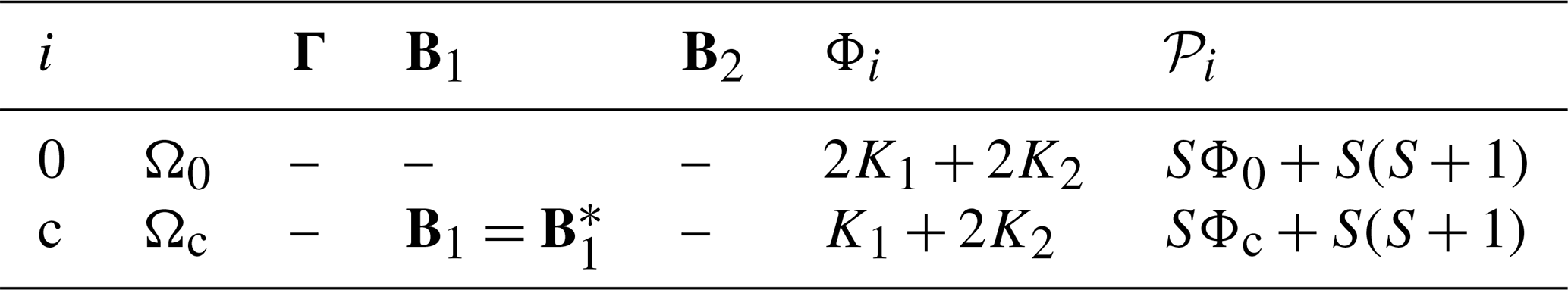
The number of parameters 𝒫 and predictors Φ associated with each hypothesis are listed in Table 1 and obtained as follows. For Eq. (5), the population parameters are ${\mathbf{B}}_{\mathrm{1}},{\mathbf{B}}_{\mathrm{2}},$ and Γ. Each B_i contains K_i predictors and therefore SK_i parameters, where $i=\mathrm{1},\mathrm{2}$. Also, Γ contains $S(S+\mathrm{1})/\mathrm{2}$ independent parameters. Equation (6) contains the same number of parameters. Therefore, the total number of parameters estimated under Ω₀ is ${\mathcal{P}}_{\mathrm{0}}=\mathrm{2}S{K}_{\mathrm{1}}+\mathrm{2}S{K}_{\mathrm{2}}+S(S+\mathrm{1})$. Under Ω_c, the complete population parameters are ${\mathbf{B}}_{\mathrm{1}},{\mathbf{B}}_{\mathrm{2}},{\mathbf{B}}_{\mathrm{2}}^{*},\mathbf{\Gamma },{\mathbf{\Gamma }}^{*}$, in particular there is only one B₁, so ${\mathcal{P}}_{\mathrm{c}}=S{K}_{\mathrm{1}}+\mathrm{2}S{K}_{\mathrm{2}}+S(S+\mathrm{1})$

The likelihood function of Eq. (5) is

$$\begin{array}{}\text{(8)}& L={\left({\displaystyle \frac{L_I}{\left(\mathrm{2}\mathit{\pi }{)}^S\right|\mathbf{\Gamma }|}}\right)}^{N/\mathrm{2}}\exp \left[-\mathbf{\Theta }/\mathrm{2}\right],\end{array}$$

where L_I is a term associated with the first P values of y_t, and

$$\mathbf{\Theta }=\mathrm{tr}\left[\left(\mathbf{Y}-{\mathbf{X}}_{\mathrm{1}}{\mathbf{B}}_{\mathrm{1}}-{\mathbf{X}}_{\mathrm{2}}{\mathbf{B}}_{\mathrm{2}}\right){\mathbf{\Gamma }}^{-\mathrm{1}}{\left(\mathbf{Y}-{\mathbf{X}}_{\mathrm{1}}{\mathbf{B}}_{\mathrm{1}}-{\mathbf{X}}_{\mathrm{2}}{\mathbf{B}}_{\mathrm{2}}\right)}^{\top }\right]$$

Similarly, the likelihood function of Eq. (6) is

$$\begin{array}{}\text{(9)}& L^{*}={\left({\displaystyle \frac{L_I^{*}}{\left(\mathrm{2}\mathit{\pi }{)}^S\right|{\mathbf{\Gamma }}^{*}|}}\right)}^{N^{*}/\mathrm{2}}\exp \left[-{\mathbf{\Theta }}^{*}/\mathrm{2}\right],\end{array}$$

where

$$\begin{array}{rl}{\mathbf{\Theta }}^{*}& =\mathrm{tr}\left[\left({\mathbf{Y}}^{*}-{\mathbf{X}}_{\mathrm{1}}^{*}{\mathbf{B}}_{\mathrm{1}}^{*}-{\mathbf{X}}_{\mathrm{2}}^{*}{\mathbf{B}}_{\mathrm{2}}^{*}\right){\left({\mathbf{\Gamma }}^{*}\right)}^{-\mathrm{1}}\right.\\ & \left.{\left({\mathbf{Y}}^{*}-{\mathbf{X}}_{\mathrm{1}}^{*}{\mathbf{B}}_{\mathrm{1}}^{*}-{\mathbf{X}}_{\mathrm{2}}^{*}{\mathbf{B}}_{\mathrm{2}}^{*}\right)}^{\top }\right]\end{array}$$

Since the noise in the two models are independent, the likelihood of both models ℒ is the product of the two individual likelihoods,

$$\mathcal{L}=L{L}^{*}.$$

The next step is to estimate the B and B^* that maximize the likelihood function under Ω₀ and under Ω_c. The resulting coefficients are called the maximum likelihood estimates (MLEs) of ${\mathbf{B}}_{{\mathrm{\Omega }}_i}$ and ${\mathbf{B}}_{{\mathrm{\Omega }}_i}^{*}$, where i=0 or c. For large N, we follow the common practice of ignoring variations in L_I and $L_I^{*}$, which corresponds to using the conditional likelihood (Box et al., 2008) (Sect. 7.1.2). Under Ω₀, the likelihoods $L_{{\mathrm{\Omega }}_{\mathrm{0}}}$ and $L_{{\mathrm{\Omega }}_{\mathrm{0}}}^{*}$ have no common parameters and therefore can be maximized separately. The resulting maximization problem is standard (e.g., Mardia et al., 1979, Chap. 6) and yields the estimates

$${\mathbf{B}}_{{\mathrm{\Omega }}_{\mathrm{0}}}={\left({\mathbf{X}}^{\top }\mathbf{X}\right)}^{-\mathrm{1}}{\mathbf{X}}^{\top }\mathbf{Y}\text{and}{\mathbf{B}}_{{\mathrm{\Omega }}_{\mathrm{0}}}^{*}={\left({\mathbf{X}}^{*\top }{\mathbf{X}}^{*}\right)}^{-\mathrm{1}}{\mathbf{X}}^{*\top }{\mathbf{Y}}^{*}.$$

and the associated degrees of freedom are

$$\begin{array}{}\text{(10)}& {\mathit{\nu }}_{{\mathrm{\Omega }}_{\mathrm{0}}}=N-K_{\mathrm{1}}-K_{\mathrm{2}}\text{and}{\mathit{\nu }}_{{\mathrm{\Omega }}_{\mathrm{0}}}^{*}=N^{*}-K_{\mathrm{1}}-K_{\mathrm{2}}.\end{array}$$

Before deriving the estimates ${\mathbf{B}}_{{\mathrm{\Omega }}_{\mathrm{c}}}$ and ${\mathbf{B}}_{{\mathrm{\Omega }}_{\mathrm{c}}}^{*}$, it is helpful to summarize the rest of the procedure presuming that these have been estimated. Specifically, the MLEs of Γ and Γ^* are

$$\begin{array}{}\text{(11)}& {\displaystyle }{\stackrel{\mathrm{‾}}{\mathbf{\Gamma }}}_{{\mathrm{\Omega }}_i}& {\displaystyle }=(\mathbf{Y}-{\mathbf{XB}}_{{\mathrm{\Omega }}_i}{)}^{\top }(\mathbf{Y}-{\mathbf{XB}}_{{\mathrm{\Omega }}_i})/N\text{(12)}& {\displaystyle }{\stackrel{\mathrm{‾}}{\mathbf{\Gamma }}}_{{\mathrm{\Omega }}_i}^{*}& {\displaystyle }=({\mathbf{Y}}^{*}-{\mathbf{X}}^{*}{\mathbf{B}}_{{\mathrm{\Omega }}_i}^{*}{)}^{\top }({\mathbf{Y}}^{*}-{\mathbf{X}}^{*}{\mathbf{B}}_{{\mathrm{\Omega }}_i}^{*})/N^{*}\end{array}$$

where i=0 or c. The deviance statistic for testing Ω₀ versus Ω_c is

$$\begin{array}{rl}{D}_{{\mathrm{\Omega }}_{\mathrm{0}:\mathrm{c}}}^{\prime }& =N\log \left|{\stackrel{\mathrm{‾}}{\mathbf{\Gamma }}}_{{\mathrm{\Omega }}_{\mathrm{c}}}\right|+N^{*}\log \left|{\stackrel{\mathrm{‾}}{\mathbf{\Gamma }}}_{{\mathrm{\Omega }}_{\mathrm{c}}}^{*}\right|-N\log \left|{\stackrel{\mathrm{‾}}{\mathbf{\Gamma }}}_{{\mathrm{\Omega }}_{\mathrm{0}}}\right|\\ & -N^{*}\log \left|{\stackrel{\mathrm{‾}}{\mathbf{\Gamma }}}_{{\mathrm{\Omega }}_{\mathrm{0}}}^{*}\right|.\end{array}$$

For sufficiently large N and N^*, the sampling distributions converge to those predicted by linear regression theory (e.g., for the univariate case, see Theorem 8.1.2 and Sect. 8.9 of Brockwell and Davis (1991) and Appendix A7.5 of Box et al. (2008); for the multivariate case, see Sect. 3.4 of Lütkepohl (2005)). Accordingly, we assume that the sample sizes are large enough for asymptotic theory to apply and therefore rely on linear regression theory for hypothesis testing in VARX models. When Ω_c is true, asymptotic theory (Hogg et al., 2019) implies that $D_{{\mathrm{\Omega }}_{\mathrm{0}:\mathrm{c}}}^{\prime }$ follows an approximate chi-squared distribution with 𝒫₀−𝒫_c degrees of freedom, specified in Table 1. In other words, if Ω_c is true, then

$$D_{{\mathrm{\Omega }}_{\mathrm{0}:\mathrm{c}}}^{\prime }\sim {\mathit{\chi }}_{{\mathcal{P}}_{\mathrm{0}}-{\mathcal{P}}_{\mathrm{c}}}^{\mathrm{2}},$$

Large values of $D_{{\mathrm{\Omega }}_{\mathrm{0}:\mathrm{c}}}^{\prime }$ lead to rejection of Ω_c.

As shown by Bartlett (1937, 1947) and discussed in Anderson (2003) (Chap. 8), the chi-squared approximation can be improved in finite samples by rescaling the deviance statistic by a factor that depends on the degrees of freedom of the underlying covariance matrices. We have explored such corrections and find that they improve the agreement with the chi-squared distribution in finite samples, but do not fully eliminate the discrepancies. We believe this limitation arises because the regression parameters are estimated by pooling samples from two populations with different covariance matrices (as shown below), so that the resulting residual covariance matrices are unlikely to follow the Wishart distribution that are assumed in the correction. Consequently, such corrections can only partially account for finite-sample effects. We find empirically that replacing N and N^* with ${\mathit{\nu }}_{{\mathrm{\Omega }}_{\mathrm{0}}}$ and ${\mathit{\nu }}_{{\mathrm{\Omega }}_{\mathrm{0}}}^{*}$, respectively, yields a modified deviance statistic that more closely matches the theoretical chi-squared distribution.

Under the above modification, the bias-corrected covariance estimates are

$$\begin{array}{}\text{(13)}& {\displaystyle }{\widehat{\mathbf{\Gamma }}}_{{\mathrm{\Omega }}_i}& {\displaystyle }=(\mathbf{Y}-\mathbf{X}{\widehat{\mathbf{B}}}_{{\mathrm{\Omega }}_i}{)}^{\top }(\mathbf{Y}-\mathbf{X}{\widehat{\mathbf{B}}}_{{\mathrm{\Omega }}_i})/{\mathit{\nu }}_{{\mathrm{\Omega }}_{\mathrm{0}}}\text{(14)}& {\displaystyle }{\widehat{\mathbf{\Gamma }}}_{{\mathrm{\Omega }}_i}^{*}& {\displaystyle }=({\mathbf{Y}}^{*}-{\mathbf{X}}^{*}{\widehat{\mathbf{B}}}_{{\mathrm{\Omega }}_i}^{*}{)}^{\top }({\mathbf{Y}}^{*}-{\mathbf{X}}^{*}{\widehat{\mathbf{B}}}_{{\mathrm{\Omega }}_i}^{*})/{\mathit{\nu }}_{{\mathrm{\Omega }}_{\mathrm{0}}}^{*}\end{array}$$

where i=0 or c, and the bias-corrected deviance statistic is

$$\begin{array}{}\text{(15)}& \begin{array}{rl}{D}_{{\mathrm{\Omega }}_{\mathrm{0}:\mathrm{c}}}& ={\mathit{\nu }}_{{\mathrm{\Omega }}_{\mathrm{0}}}\log \left|{\widehat{\mathbf{\Gamma }}}_{{\mathrm{\Omega }}_{\mathrm{c}}}\right|+{\mathit{\nu }}_{{\mathrm{\Omega }}_{\mathrm{0}}}^{*}\log \left|{\widehat{\mathbf{\Gamma }}}_{{\mathrm{\Omega }}_{\mathrm{c}}}^{*}\right|-{\mathit{\nu }}_{{\mathrm{\Omega }}_{\mathrm{0}}}\log \left|{\widehat{\mathbf{\Gamma }}}_{{\mathrm{\Omega }}_{\mathrm{0}}}\right|\\ & -{\mathit{\nu }}_{{\mathrm{\Omega }}_{\mathrm{0}}}^{*}\log \left|{\widehat{\mathbf{\Gamma }}}_{{\mathrm{\Omega }}_{\mathrm{0}}}^{*}\right|.\end{array}\end{array}$$

If Ω_c is true, then

$$\begin{array}{}\text{(16)}& D_{{\mathrm{\Omega }}_{\mathrm{0}:\mathrm{c}}}\sim {\mathit{\chi }}_{{\mathcal{P}}_{\mathrm{0}}-{\mathcal{P}}_{\mathrm{c}}}^{\mathrm{2}}.\end{array}$$

It remains to obtain the maximum likelihood estimates under Ω_c. It proves convenient to express the likelihood in terms of a common set of regression coefficients

$$\begin{array}{}\text{(17)}& \mathbb{B}=\left[\begin{array}{c}{\mathbf{B}}_{\mathrm{1}}\\ {\mathbf{B}}_{\mathrm{2}}\\ {\mathbf{B}}_{\mathrm{2}}^{*}\end{array}\right].\end{array}$$

There is no loss in generality in omitting the 2π terms in the likelihoods (because they cancel after computing the ratio) and by considering the logarithm of the likelihood (since the logarithm transformation does not change the location of the maximum). Also, as discussed earlier, the terms L_I and $L_I^{*}$ are ignored. With these considerations, the log-likelihood (times −2) becomes

$$\begin{array}{}\text{(18)}& -\mathrm{2}\log {\mathcal{L}}_{{\mathrm{\Omega }}_{\mathrm{c}}}={\mathit{\nu }}_{{\mathrm{\Omega }}_{\mathrm{0}}}\log \left|\mathbf{\Gamma }\right|+{\mathit{\nu }}_{{\mathrm{\Omega }}_{\mathrm{0}}}^{*}\log \left|{\mathbf{\Gamma }}^{*}\right|+\mathbf{\Theta }+{\mathbf{\Theta }}^{*},\end{array}$$

where in this notation

$$\begin{array}{ll}{\displaystyle }\mathbf{\Theta }& {\displaystyle }=\mathrm{tr}\left[\left(\mathbf{Y}-\mathbb{X}\mathbb{B}\right){\left(\mathbf{\Gamma }\right)}^{-\mathrm{1}}{\left(\mathbf{Y}-\mathbb{X}\mathbb{B}\right)}^{\top }\right]\\ {\displaystyle }{\mathbf{\Theta }}^{*}& {\displaystyle }=\mathrm{tr}\left[\left({\mathbf{Y}}^{*}-{\mathbb{X}}^{*}\mathbb{B}\right){\left({\mathbf{\Gamma }}^{*}\right)}^{-\mathrm{1}}{\left({\mathbf{Y}}^{*}-{\mathbb{X}}^{*}\mathbb{B}\right)}^{\top }\right],\end{array}$$

and where

$$\begin{array}{ll}{\displaystyle }\mathbb{X}& {\displaystyle }=\left[\begin{array}{ccc}{\mathbf{X}}_{\mathrm{1}}& {\mathbf{X}}_{\mathrm{2}}& \mathbf{0}\end{array}\right]\\ {\displaystyle }{\mathbb{X}}^{*}& {\displaystyle }=\left[\begin{array}{ccc}{\mathbf{X}}_{\mathrm{1}}^{*}& \mathbf{0}& {\mathbf{X}}_{\mathrm{2}}^{*}\end{array}\right].\end{array}$$

Differentiating with respect to 𝔹 yields

$$\begin{array}{rl}{\displaystyle \frac{\partial }{\partial \mathbb{B}}}\left(-\mathrm{2}\log {\mathcal{L}}_{{\mathrm{\Omega }}_{\mathrm{c}}}\right)& =-\mathrm{2}{\mathbb{X}}^{\top }\left(\mathbf{Y}-\mathbb{X}\mathbb{B}\right){\left(\mathbf{\Gamma }\right)}^{-\mathrm{1}}\\ & -\mathrm{2}{\mathbb{X}}^{*T}\left({\mathbf{Y}}^{*}-{\mathbb{X}}^{*}\mathbb{B}\right){\left({\mathbf{\Gamma }}^{*}\right)}^{-\mathrm{1}}.\end{array}$$

Setting this to zero and manipulating yields

$${\mathbb{X}}^{\top }\mathbf{Y}{\mathbf{\Gamma }}^{-\mathrm{1}}+{\mathbb{X}}^{*T}{\mathbf{Y}}^{*}{\mathbf{\Gamma }}^{*-\mathrm{1}}={\mathbb{X}}^{\top }\mathbb{X}\mathbb{B}{\mathbf{\Gamma }}^{-\mathrm{1}}+{\mathbb{X}}^{*T}{\mathbb{X}}^{*}\mathbb{B}{\mathbf{\Gamma }}^{*-\mathrm{1}},$$

which is a linear matrix equation for 𝔹 whose solution is known (Lancaster, 1970). A straightforward solution method is to use the following standard identity for any three matrices $\mathbf{A},\mathbf{B},\mathbf{C}$:

$$\text{vec}\left[\mathbf{ABC}\right]=({\mathbf{C}}^{\top }\otimes \mathbf{A})\text{vec}\left[\mathbf{B}\right],$$

where vec[B] is a column vector obtained by stacking the columns of B, and ⊗ is the Kronecker product (Seber, 2008, Sect. 11.16). The final result is

$$\begin{array}{}\text{(19)}& \begin{array}{rl}\text{vec}\left[\widehat{\mathbb{B}}\right]& ={\left({\mathbf{\Gamma }}^{-\mathrm{1}}\otimes {\mathbb{X}}^{\top }\mathbb{X}+{\mathbf{\Gamma }}^{*-\mathrm{1}}\otimes {\mathbb{X}}^{*T}{\mathbb{X}}^{*}\right)}^{-\mathrm{1}}\\ & \text{vec}\left[{\mathbb{X}}^{\top }\mathbf{Y}{\mathbf{\Gamma }}^{-\mathrm{1}}+{\mathbb{X}}^{*T}{\mathbf{Y}}^{*}{\mathbf{\Gamma }}^{*-\mathrm{1}}\right],\end{array}\end{array}$$

where the inverse exists because the Kronecker product of positive definite matrices is positive definite, and the sum of positive definite matrices is positive definite (and of course positive definite matrices are invertible). Maximizing the modified likelihood with respect to Γ and Γ^* yields Eq. (13) and Eq. (14), where ${\mathbf{B}}_{{\mathrm{\Omega }}_{\mathrm{c}}}$ and ${\mathbf{B}}_{{\mathrm{\Omega }}_{\mathrm{c}}}^{*}$ are extracted from $\widehat{\mathbb{B}}$ as defined in Eq. (17). Equations  (13),  (14),  (19) define a set of nonlinear equations whose solution requires iterative methods. To start the iteration, we use the regression coefficients for equal noise covariances, which can be solved directly as

$${\widehat{\mathbb{B}}}_{\mathrm{\Gamma }={\mathrm{\Gamma }}^{*}}={\left({\mathbb{X}}^{\top }\mathbb{X}+{\mathbb{X}}^{*T}{\mathbb{X}}^{*}\right)}^{-\mathrm{1}}\left({\mathbb{X}}^{\top }\mathbf{Y}+{\mathbb{X}}^{*T}{\mathbf{Y}}^{*}\right).$$

This solution is substituted into Eqs. (13) and (14) to obtain updated estimates of the noise covariance matrices, which in turn are substituted into Eq. (19) to obtain a new estimate of 𝔹. These steps are repeated until convergence. Convergence is monitored using the log-likelihood Eq. (18). Empirically, by the fourth iteration the relative change in log-likelihood is less than 1 % for 97 % of all pairwise comparisons. This finding indicates that the iterative scheme is stable and rapidly convergent in practice, although a formal theoretical analysis of its convergence properties is beyond the scope of this study. Given the consistently rapid convergence observed, we terminate the algorithm after four iterations. Codes for performing this test are publicly available (see code availability statement).

3 Monte Carlo Simulations

In this section, we apply the above test and assess how well the theoretical chi-squared distribution is realized in practice. Our strategy is to generate simulations from two VARX models whose parameters satisfy a given hypothesis. Then, the deviance between time series is computed from multiple realizations to derive an empirical distribution of the deviances, which is compared with the corresponding theoretical distribution Eq. (16). This approach requires specifying numerical values for the VARX parameters. To ensure that the values used in the tests are representative of those that might be encountered in climate applications, we estimate VARX models from observations and climate simulations.

Monthly mean 2 m air temperature is selected for analysis. This choice is supported by a long history of using autoregressive models to simulate temperature variability (Leith, 1973) and predict temperature on monthly-to-decadal time scales (Penland and Sardeshmukh, 1995; Newman, 2013). Here, global temperature fields are spatially aggregated into S=5 broad regions, illustrated in Fig. 1. These regions are derived from the climatologically consistent regions defined by Iturbide et al. (2020a), but are aggregated according to location (tropical, Northern Hemisphere, or Southern Hemisphere) and surface type (land or ocean). Aggregation of temperature over large spatial regions is expected to enhance Gaussianity through the central limit theorem. While there is evidence that temperature variability exhibits non-Gaussian structure (Sardeshmukh and Penland, 2015), and that such behavior can be captured using appropriate nonlinear extensions of autoregressive models, these extensions are not considered here.

Figure 1 The five spatial domains over which monthly mean 2 m air temperature is averaged. White areas over the Mediterranean and selected tropical land regions are excluded from the analysis.

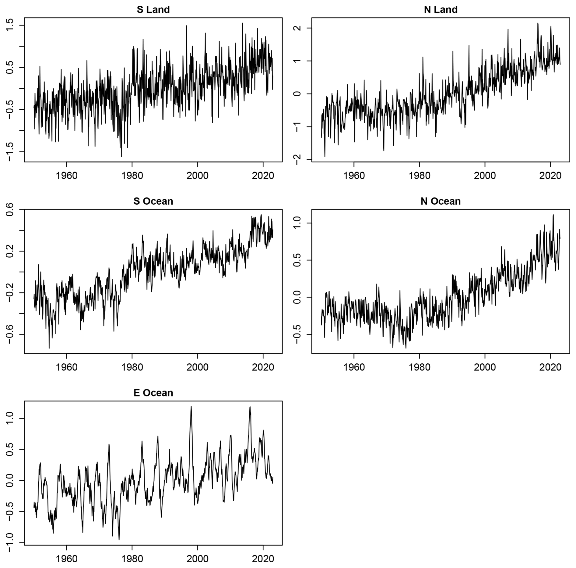
Figure 2 Anomaly time series of ERA5 2 m temperature averaged over the five spatial regions shown in Fig. 1. Anomalies are computed with respect to the monthly climatology over 1950–2014.

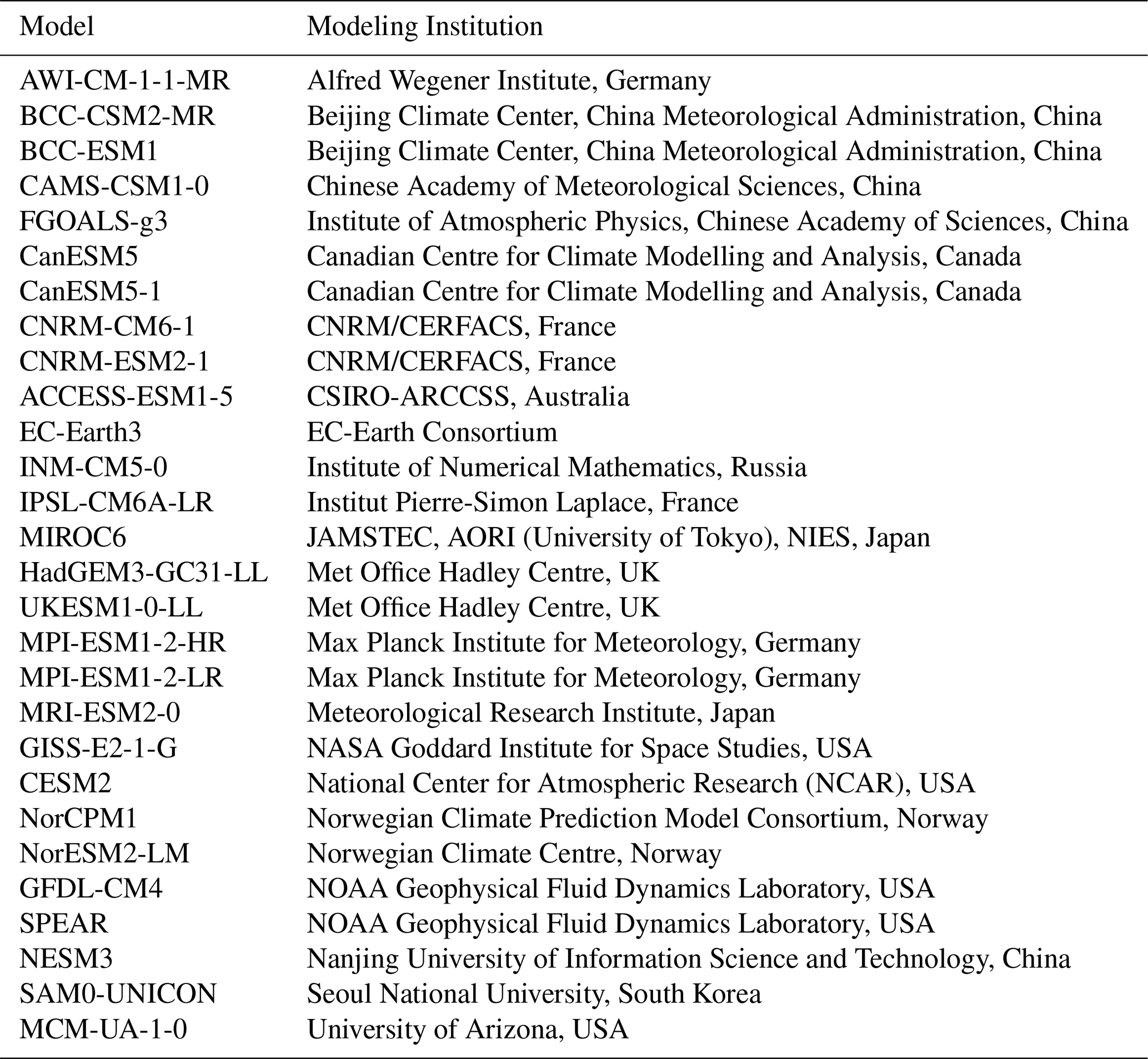
For observational data, we use monthly 2 m air temperature from the ERA5 reanalysis (Hersbach et al., 2020). Time series of this variable averaged over the five analysis regions are shown in Fig. 2 and exhibit clear warming trends. For simulations, we use monthly 2 m air temperature from historical simulations conducted as part of the Coupled Model Intercomparison Project Phase 6 (CMIP6; Eyring et al., 2016). We also have included the SPEAR model from the Geophysical Fluid Dynamics Laboratory (Delworth et al., 2020). These simulations cover the 165-year period 1850–2014 and are driven by radiative forcing from natural and anthropogenic sources, with magnitudes constrained by historical observations. A total of 27 distinct models were selected, representing one model from each participating modeling center, with a single ensemble member retained for each model. The selected models are listed in Table 2. The simulated global fields are aggregated to the same five spatial regions defined in Fig. 1, allowing direct comparison with the corresponding observations.

The available observations and simulations span different time periods. Although the test does not require equal sample sizes, comparisons across non-overlapping periods complicate interpretation, since detected differences could reflect nonstationary changes rather than differences in model parameters. To avoid this ambiguity, we restrict the analysis to a common time interval. In addition, only observational data after January 1950 are considered in order to avoid known data quality issues prior to this date (Chan et al., 2019). The resulting ERA5 observations and CMIP6 historical simulations overlap over the 65-year period 1950–2014, and all analyses are therefore confined to this interval. This choice corresponds to 780 months, and hence $N=N^{*}=\mathrm{780}-P$.

Table 2 List of CMIP6 models and their modeling institutions.

To represent changes in radiative forcing from evolving atmospheric composition, we use the estimates provided in Table A3.4 of Annex III in the latest IPCC report (Dentener et al., 2021). Specifically, we include anthropogenic aerosols (“Aerosols”), natural forcings (“Natural”), and the residual obtained by subtracting these two from the total forcing, which is dominated by well-mixed greenhouse gases (“WMGHG”). The forcing data are annual means and were linearly interpolated to monthly resolution for use in this study (Fig. 3). We also include six annual harmonics to represent the seasonal cycle, along with an intercept term for the climatological mean, giving 12 seasonal forcing functions in total (note that this variability was removed to make Fig. 2). Combined with the three radiative forcing terms, this yields J=15 forcing functions.

Figure 3 Effective Radiative Forcings (ERFs) used in the autoregressive models. The forcings include greenhouse gases (WMGHG), anthropogenic aerosols, and natural forcings (e.g., volcanoes and solar variability).

To select the model order, we use the Mutual Information Criterion (MIC; DelSole and Tippett, 2021b), which selects P=1 or P=2 for ERA5 and most CMIP6 models. In general, it is preferable to slightly overfit rather than underfit. Underfitting can leave residual serial correlation, violating the independence assumption required for deriving the sampling distributions of the deviance statistic. Overfitting, by contrast, typically yields white-noise residuals, albeit at the cost of increased variance in the parameter estimates. Importantly, the added uncertainty due to overfitting is explicitly accounted for in the likelihood ratio test. From the perspective of this study, the main drawback of overfitting is the loss of statistical power; i.e., increased probability of failing to reject a false hypothesis (i.e., the likelihood of false negatives). Consequently, model differences must be relatively large to remain detectable when overfitting is present. As will be shown below, these are not serious concerns in this study. For these reasons, as well as considerations of simplicity and consistency, we adopt P=2 for all cases.

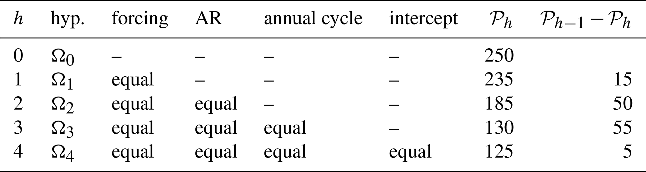
With the above choices, we obtain a VARX model of the form Eq. (1) with $S=\mathrm{5},P=\mathrm{2},J=\mathrm{15}$. The choice of which subset of VARX parameters to test depends on the study's objectives. For example, studies focused on internal variability may test for differences in AR coefficients, whereas studies concerned with forced variability may test for differences in transfer coefficients. Our framework is general and can accommodate any subset of coefficients. For the analyses presented here, we test the hypotheses listed in Table 3. For each hypothesis h, the VARX parameters under Ω_h are obtained as described in Sect. 2 using ERA5 data and a single CMIP6 simulation. This yields a pair of VARX models with different noise covariances, while the remaining parameters are either equal or different according to the specification of Ω_h. For context, we find that the noise variances in observations and simulations (i.e., the diagonal elements of the noise covariance matrices Γ and Γ^*) differ by up to a factor of eight for a given spatial domain (not shown). These differences are not claimed to be statistically significant; rather, they give context for the magnitude of heterogeneity of noise variances encountered in practical applications.

Table 3 Summary of the hypotheses for comparing parameters across two VARX models with different noise covariances. “Equal” indicates that the corresponding parameter is equal between two VARX models, and a hyphen indicates that the corresponding parameter is unrestricted. “Forcing” indicates the transfer coefficients for GHG, AER, NAT forcings; “AR” denotes the AR parameters ${\mathbf{A}}_{\mathrm{1}},\mathrm{\dots },{\mathbf{A}}_p$; “annual cycle” denotes the coefficients of the annual harmonics; “intercept” denotes the constant intercept coefficient.

The question arises as to how to generate simulations that contain both forced and internal variability specific to the 1950–2014 period. An efficient strategy exploits the linearity of the VARX model. Specifically, we compute the internal and forced components separately, then sum them to obtain the 1950–2014 solution. The internal component is generated by integrating the VAR model without exogenous forcing from an arbitrary initial state, discarding the first 65 years to remove transient spin-up, and then continuing the run to produce a long record. Consecutive 65-year segments are extracted as realizations of internal variability. The forced component is obtained by integrating the noise-free VARX model from 1750 (the start of the forcing data) to 2014, again from an arbitrary initial state. Because the system is damped, all memory of the initial condition vanishes by 1950, and since the forcing is deterministic, this integration needs to be performed only once to obtain the forced component. Finally, each 65-year segment of internal variability is combined with the 1950–2014 segment of the forced run to generate realizations containing both forced and internal variability, which are then used to compute the deviance.

In what follows, we present results for Ω₄. A key advantage of simulating under Ω₄ is that the other hypotheses Ω₁, Ω₂, and Ω₃ are also true by construction, allowing them to be tested separately using the same simulations. We have conducted separate simulations under Ω₁, Ω₂, Ω₃, but the results are sufficiently similar to those for Ω₄ that they are not shown. We generate simulations of internal variability that are 1000 times longer than the original time series. Each consecutive 65-year segment is combined with the 1950–2014 solution from the forced variability run, producing 1000 synthetic 65-year segments containing both forced and internal variability. This enables the comparison test to be performed 1000 times, yielding 1000 deviance values under the specified hypothesis. Implementing this procedure requires integrating the VARX model to simulate approximately 65 000 years for each CMIP6 model and 65 000 years for ERA5. Repeating the process for all 27 models produces a total of roughly 3.5 million simulated years from the VARX model. These computations were relatively inexpensive: the full set of simulations was completed in a few hours on a standard MacBook Pro.

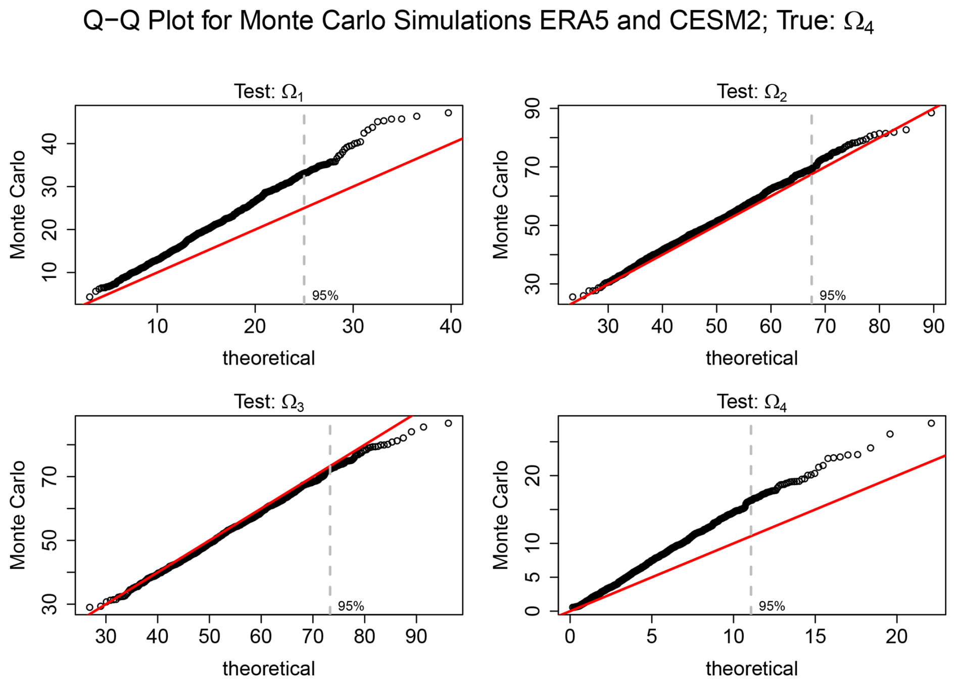
Figure 4 Q–Q plots comparing deviances from Monte Carlo simulations with the corresponding theoretical chi-squared distribution for the hypotheses Ω₁, Ω₂, Ω₃, and Ω₄ defined in Table 3. The red line denotes the 1:1 reference, and the dashed grey vertical line marks the 95 % critical value of the chi-squared distribution under each hypothesis. The degrees of freedom for comparing Ω_h to Ω_h−1 are given by $({\mathcal{P}}_{h-\mathrm{1}}-{\mathcal{P}}_h)$, as listed in Table 3.

A Q–Q plot comparing deviance values with the corresponding theoretical chi-squared distribution for a specific model (CESM2) is shown in Fig. 4. The chi-squared distribution is closely followed for Ω₂ and Ω₃, as indicated by the close alignment of the points with the 1:1 reference line. In contrast, for Ω₁ and Ω₄, the theoretical distribution tends to underestimate the upper quantiles of the Monte Carlo simulations. The latter two hypotheses also have relatively few degrees of freedom compared to the others (see Table 3), suggesting a potential bias when the degrees of freedom are small.

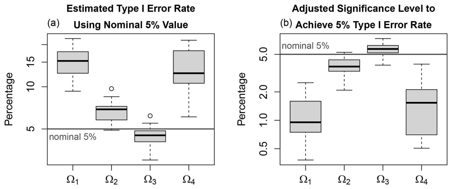
Figure 5 Type I error statistics of tests of hypotheses ${\mathrm{\Omega }}_{\mathrm{1}},{\mathrm{\Omega }}_{\mathrm{2}},{\mathrm{\Omega }}_{\mathrm{3}},{\mathrm{\Omega }}_{\mathrm{4}}$ (defined in Table 3) estimated from Monte Carlo simulations of 27 VARX models trained on CMIP6 simulations. (a) Empirical Type I error rates obtained using the nominal chi-squared critical value at the 5 % significance level. Box-and-whisker plots summarize results across CMIP6 simulations: boxes indicate the interquartile range, thick lines denote the median, whiskers extend to 1.5 times the interquartile range, and circles indicate outliers. (b) Adjusted significance levels in the chi-squared distribution required to achieve an empirical 5 % Type I error rate, as estimated from the Monte Carlo experiments discussed in the text. Note that the y-axis have different ranges and are shown on a logarithmic scale.

Results for the remaining models follow the pattern illustrated in Fig. 4: the theoretical chi-squared distribution tends to underestimate the upper quantiles for Ω₁ and Ω₄, while providing a reasonable approximation for Ω₂ and Ω₃ (not shown). To quantify these discrepancies more precisely, Fig. 5a shows the empirical Type I error rates across models when the 5 % critical value from the chi-squared distribution is used. For each model, the Type I error rate is computed as the fraction of Monte Carlo samples whose deviance exceeds the 5 % critical value from the chi-squared distribution. For Ω₁, Ω₂, and Ω₄, the empirical Type I error rates generally exceed the 5 % level, reaching values as high as 20 % in some cases. Thus, when the theoretical distribution is used for these hypotheses, the probability of falsely rejecting the null hypothesis is higher than intended. In practical terms, the test may identify significant differences in VARX parameters more frequently than warranted when the null hypothesis is true. This bias can be partially mitigated by reducing the significance level in the chi-squared distribution. Figure 5b shows the adjusted significance levels in the chi-squared distribution required to achieve an empirical 5 % Type I error rate for each model. These adjusted levels are obtained by estimating the 95th percentile of the deviance statistic from the Monte Carlo simulations and then computing the corresponding p-value under the theoretical chi-squared distribution. The resulting adjusted significance levels are typically in the range 0.5 %–2 %, indicating that applying the test at these more stringent levels yields Type I error rates closer to the intended 5 %. For Ω₃, the discrepancy has the opposite sign: the empirical Type I error rate is slightly below the intended 5 % level, although the deviation is comparatively small.

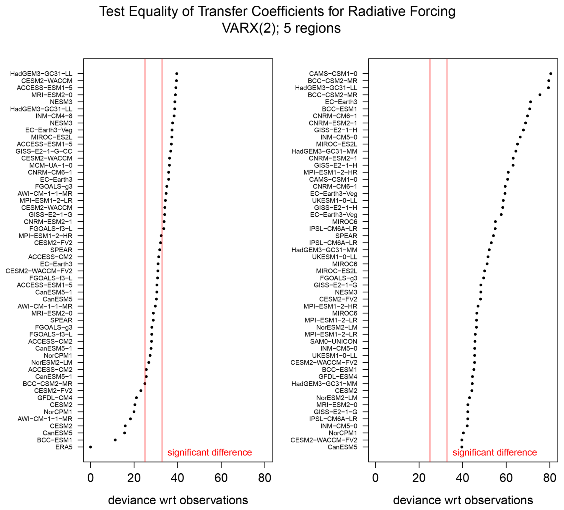
Figure 6 The deviance statistic for testing equality of transfer coefficients for radiative forcing between observations (ERA5) and each CMIP6 simulation of monthly 2 m-temperature over 1950–2014. The results are spread across two panels. The temperature field is represented by the five domains shown in Fig. 1. The left and right red lines denote the 5 % and 0.5 % significance thresholds, respectively; points to the right indicate significant deviances, meaning that a significant difference in the corresponding VARX parameter was detected at the prescribed significance level. Models are ordered by their deviance values, with individual ensemble members listed separately when available.

Figure 7 Same as Fig. 6, but for testing equality of AR coefficients.

4 Comparing CMIP6 Simulations to Observations

We now apply the proposed test to assess if CMIP6 simulations are statistically distinguishable from observations. For this analysis, we include all available climate models, allowing multiple models from the same center and up to three ensemble members per model, for a total of 108 simulations. Our focus is on whether the simulations produce realistic internal variability and responses to external forcing, which are governed by the AR coefficients and the transfer coefficients for radiative forcing.

The results of testing equality of transfer coefficients associated with radiative forcing between ERA5 and the CMIP6 simulations are shown in Fig. 6. Using the nominal significance level of 5 %, approximately 90 % of the CMIP6 models exhibit statistically significant deviance values, indicating that transfer coefficients differ significantly from those inferred from observations for the majority of models. When accounting for a potential bias in Type I error by adopting a more stringent significance level of 0.5 %, differences in transfer coefficients still are detected in 72 % of the CMIP6 models. In both cases, the number of detected differences far exceeds the nominal 5 % rate expected if CMIP6 models were consistent with observations.

Note that each hypothesis test is interpreted individually and the reported fractions of rejections are compared against the expected Type I error rate. No global hypothesis across models is being tested. The purpose of the analysis is to document model-by-model differences relative to observations, as is common in model evaluation studies. If one were instead testing a global null hypothesis that all models are consistent with observations, then multiple-testing adjustments would be required.

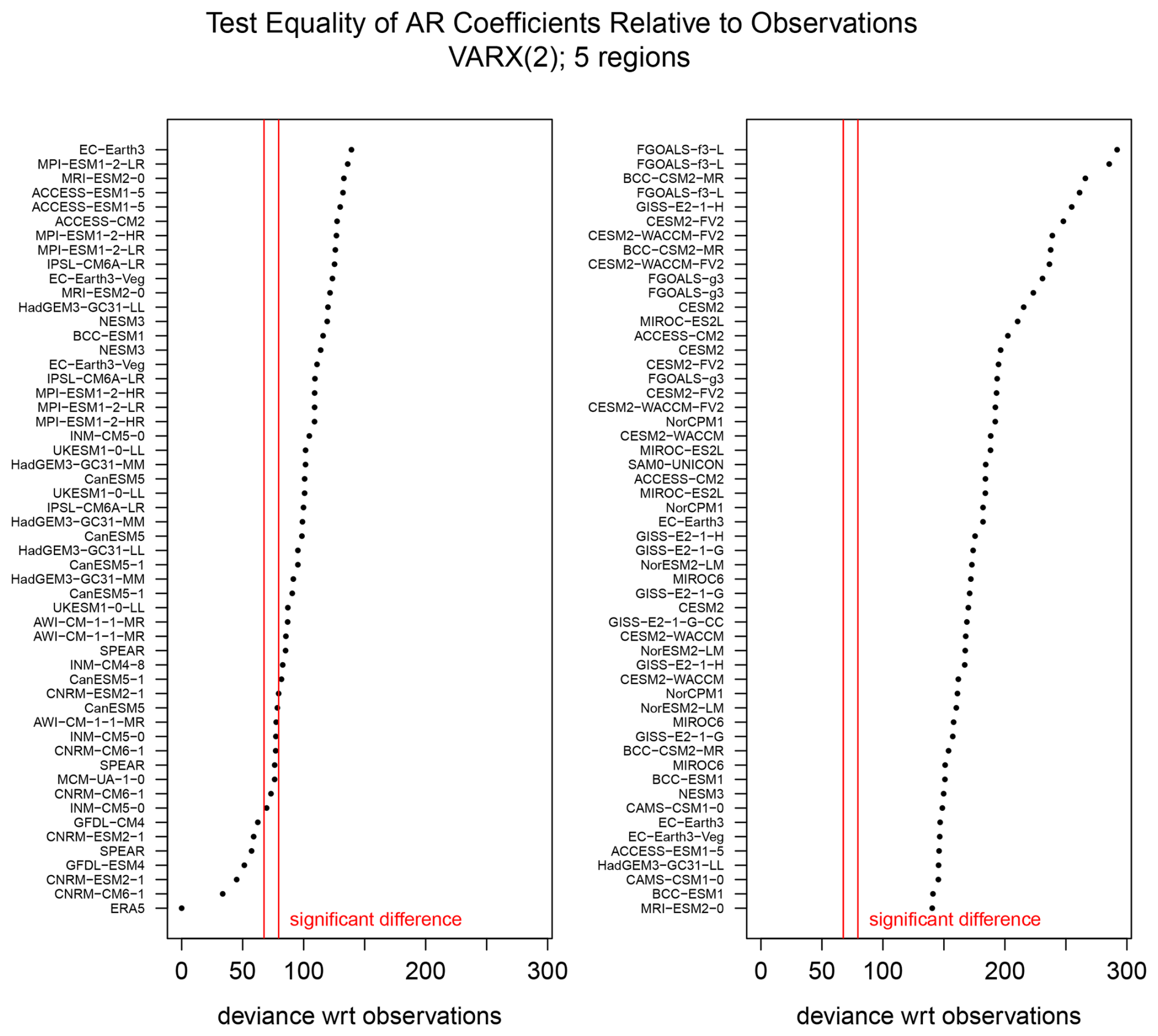
The results of testing equality of AR coefficients between observations and CMIP6 simulations are shown in Fig. 7. In this case, 94 % of the CMIP6 models have deviances that exceed the nominal 5 % significance level, and 87 % of the models exceed the threshold for 0.5 % significance. In both cases, the number of detected differences in AR coefficients far exceeds the expected Type I error rate of 5 % if the CMIP6 models were consistent with observations. When both AR coefficients and radiative transfer coefficients are tested, every CMIP6 model exhibits significant deviances from observations (not shown).

The VARX specification may not capture all relevant forcings present in observations and CMIP6 simulations. In such cases, omitted common forcings could induce cross-correlation between the residuals of the two fitted models. To assess this possibility, we examined cross-correlations of VARX residuals pooled across the five regions and 108 time series (28 890 pairwise correlations, not all independent). The empirical 5–95 percentile range of correlations is (−0.051, 0.100). These magnitudes are small and correspond to less than 1 % of the variance (i.e., r²≤0.01), providing no evidence of substantial residual dependence attributable to omitted common forcings.

5 Summary and Conclusions

This study developed and applied a statistical method for rigorously comparing the parameters of Vector Autoregressive models with exogenous inputs (VARX) trained on climate model simulations and observations. The approach extends methods developed in our previous work (DelSole and Tippett, 2020, 2021a, 2022a, b, 2024) by removing the requirement of equal noise covariances. As such, the new method allows more targeted subsets of model parameters to be compared, enabling direct investigation of which statistical features differ between two time series. An important application is to determine if two time series share the same predictability or memory characteristics. In univariate models, these properties are governed by the time-lagged correlations, which depend solely on the autoregressive coefficients, and hence could be compared by testing the equality of AR coefficients independently of differences in noise variance. A complementary application is to determine if two time series exhibit the same co-variability with external forcing. In VARX models, this property is governed by the transfer coefficients and likewise requires testing their equality without assuming identical noise structure.

The test is based on the likelihood ratio, with an iterative method to solve the resulting nonlinear system of equations. Monte Carlo experiments reveal that, for large degrees of freedom, the test statistic follows an approximate chi-squared distribution as predicted by asymptotic theory. For small degrees of freedom, the Type I error rate tends to be inflated; for instance, for a prescribed 5 % significance level, the empirical Type I error rate often was higher, reaching about 20 %. This bias is correctable to some extent by adjusting the nominal significance level from 5 % to 0.5 %–2 % (see Fig. 5b). In applications where more accurate control of Type I error is required, bootstrap-based calibration of critical values may provide a useful refinement.

Applying the method to monthly 2m-temperature data from ERA5 and historical CMIP6 simulations revealed that over 90 % of the CMIP6 models have transfer coefficients and AR coefficients that differ from those inferred from observations at the 5 % significance level. Adopting more stringent significance levels to compensate for the potentially biased Type I error rate still leads to detectable differences in the AR parameters and transfer coefficients in at least three quarters of the CMIP6 models. Moreover, none of the CMIP6 models examined are consistent with ERA5 in both the autoregressive and transfer coefficients. Discrepancies in these parameters are particularly important because they govern how the VARX model responds to anomalous forcing. Taken together, these results suggest that many current CMIP6 models exhibit systematic differences from ERA5 in their simulated responses to enhanced radiative forcing.

Beyond the application considered here, the proposed framework is broadly applicable to climate variables that are well represented by low-dimensional VARX models, which encompasses many quantities that are routinely analyzed using Linear Inverse Models and related stochastic-dynamical approaches. While the examples in this study are based on regional averages, the proposed framework extends naturally to spatiotemporal fields through suitable dimension reduction, for example to the leading principal components of spatial fields or to multivariate state vectors comprising physically distinct variables with different units. A key assumption is that the dominant external forcings are known and explicitly included in the VARX formulation. If an important forcing that affects one data set is omitted from the model, the associated forced signal may be misattributed to internal variability or manifest as residual correlations across data sets, thereby violating the assumed independence of the residuals. The framework is further restricted to Gaussian processes of modest dimension and may be less suitable for variables exhibiting pronounced nonlinearities, regime behavior, long-memory properties, or heteroskedasticity. Several of these assumptions can be relaxed through model extensions; for example, the framework can be generalized to cyclostationary processes, which would further expand its applicability to seasonally varying climate dynamics.