the Creative Commons Attribution 4.0 License.
the Creative Commons Attribution 4.0 License.
 | 12 Oct 2020
Comparing climate time series – Part 1: Univariate test
Michael K. Tippett
This paper proposes a new approach to detecting and describing differences in stationary processes. The approach is equivalent to comparing auto-covariance functions or power spectra. The basic idea is to fit an autoregressive model to each time series and then test whether the model parameters are equal. The likelihood ratio test for this hypothesis has appeared in the statistics literature, but the resulting test depends on maximum likelihood estimates, which are biased, neglect differences in noise parameters, and utilize sampling distributions that are valid only for large sample sizes. This paper derives a likelihood ratio test that corrects for bias, detects differences in noise parameters, and can be applied to small samples. Furthermore, if a significant difference is detected, we propose new methods to diagnose and visualize those differences. Specifically, the test statistic can be used to define a “distance” between two autoregressive processes, which in turn can be used for clustering analysis in multi-model comparisons. A multidimensional scaling technique is used to visualize the similarities and differences between time series. We also propose diagnosing differences in stationary processes by identifying initial conditions that optimally separate predictable responses. The procedure is illustrated by comparing simulations of an Atlantic Meridional Overturning Circulation (AMOC) index from 10 climate models in Phase 5 of the Coupled Model Intercomparison Project (CMIP5). Significant differences between most AMOC time series are detected. The main exceptions are time series from CMIP models from the same institution. Differences in stationary processes are explained primarily by differences in the mean square error of 1-year predictions and by differences in the predictability (i.e., R-square) of the associated autoregressive models.


Climate scientists often confront questions of the following types.
-
Does a climate model realistically simulate a climate index?
-
Do two climate models generate similar temporal variability?
-
Did a climate index change its variability?
-
Are two power spectra consistent with each other?
Each of the above questions requires deciding whether two time series come from the same stochastic process. Although numerous papers in the weather and climate literature address questions of the above types, the conclusions often are based on visual comparison of estimated auto-covariance functions or power spectra without a rigorous significance test. Lund et al. (2009) provide a lucid review of some objective tests for deciding whether two time series come from the same stationary process. An additional test that was not considered by Lund et al. (2009) is to fit autoregressive models to time series and then to test differences in parameters (Maharaj, 2000; Grant and Quinn, 2017). Grant and Quinn (2017) showed that this test has good power and performs well even when the underlying time series are not from an autoregressive process. The latter test has been applied to such problems as speech recognition but not to climate time series. The purpose of this paper is to further develop this test for climate applications.
The particular tests proposed by Maharaj (2000) and Grant and Quinn (2017) test equality of autocorrelation without regard to differences in variances. However, in climate applications, differences in variance often are of considerable importance. In addition, these tests employ a sampling distribution derived from asymptotic theory and therefore may be problematic for small sample sizes. In this paper, the likelihood ratio test is derived for the more restrictive case of equality of noise variances, which leads to considerable simplifications, including a test that is applicable for small sample sizes. Further comments about how our proposed test compares with previous tests will be discussed below.
If the time series are deemed to come from different processes, then it is desirable to characterize those differences in meaningful terms and to group time series into clusters. Piccolo (1990) and Maharaj (2000) propose such classification procedures. Following along these lines, our hypothesis test suggests a natural measure for measuring the distance between two stationary processes that can be used for clustering analysis. For multi-model studies, this distance measure can be used to give a graphical summary of the similarities and differences between time series generated by different models. In addition, we extend the interpretation of such summaries considerably by proposing a new approach to diagnosing differences in stationary processes based on finding the initial condition that optimally separates one-step predictions.
In this section we review previous methods for comparing two time series. These methods are based on the theory of stochastic processes and assume that the joint distribution of the values of the process at any collection of times is multivariate normal and stationary. Although non-stationarity is a prominent feature in many climate time series, a stationary framework is a natural starting point for non-stationary generalizations. Stationarity implies that the expectation at any time is constant, and the second-order moments depend only on the difference times (more precisely, this is called weak-sense stationarity). Accordingly, if Xt is a stationary process, then the mean is independent of time,
and the time-lagged auto-covariance function depends only on the difference in times,
Because a multivariate normal distribution is fully characterized by its first and second moments, the stochastic process is completely specified by μX and the auto-covariance function cX(τ). Stationarity further implies that the auto-covariance function is an even function of the lag τ. Following standard practice, we consider discrete time series where values are available at NX equally spaced time steps .
Now consider another stationary process Yt, with mean μY and auto-covariance function cY(τ). The problem we consider is this: given sample time series and , decide whether the two time series come from the same stationary process. For stationary processes, we often are not concerned with differences in means (e.g., in climate studies, these often are eliminated through “bias corrections”), hence we allow μX≠μY. Therefore, our problem is equivalent to deciding whether the two time series have the same auto-covariance function, i.e., deciding whether
This problem can be framed equivalently as deciding whether two stationary processes have the same power spectrum. Recall that the power spectrum is the Fourier transform of the auto-covariance function. We define the power spectrum of Xt as
The spectrum of Yt is defined similarly and denoted as pY(ω). Because the Fourier transform is invertible, equality of auto-covariances is equivalent to equality of spectra. Thus, our problem can be framed equivalently as deciding whether
Estimates of the power spectrum are based on the periodogram (Box et al., 2008).
The above hypothesis differs from hypotheses about a single process that are commonly tested with auto-covariance functions or power spectra. For instance, the hypothesis of vanishing auto-correlation often is assessed by comparing the sample auto-correlation function to , where N is the length of the time series (e.g., Brockwell and Davis, 2002, chap. 1). In the spectral domain, the hypothesis of white noise often is tested based on the Kolmogorov–Smirnov test, in which the standardized cumulative periodogram is compared to an appropriate set of lines (e.g., Jenkins and Watts, 1968, Sect. 6.3.2). These tests consider hypotheses about one process. In contrast, our hypothesis involves a comparison of two processes.
Coates and Diggle (1986) derived spectral-domain tests for equality of stationary processes. The underlying idea of these tests is that equality of power spectra implies that their ratio is independent of frequency and therefore indistinguishable from white noise. This fact suggests that standard tests for white noise can be adapted to periodogram ratios. Coates and Diggle (1986) derive a second parametric test that assumes that the log ratio of power spectra is a low-order polynomial of frequency.
Lund et al. (2009) explored the above tests in the context of station data for temperature. They found that spectral methods have relatively low statistical power – that is, the methods are unlikely to detect a difference in stationary processes when such a difference exists. Our own analysis using the data discussed in Sect. 5 is consistent with Lund et al. (2009) (not shown). The fact that spectral-domain tests have less statistical power than time-domain tests is not surprising. After all, spectral tests are based on comparing periodograms in which the number of unknown parameters grows with sample size. In particular, for a time series of length N, the periodogram combines coefficients for sines and cosines of a Fourier transform into N∕2 coefficients for the amplitude. Thus, a time series of length N=64 yields a periodogram with 32 amplitudes; a time series of length N=512 yields a periodogram with 256 amplitudes; and so on. Because the number of unknowns grows with sample size, the sampling error of the individual periodogram estimates does not decrease with sample size. Typically, sampling errors are reduced by smoothing periodogram estimates over frequencies, but the smoothing makes implicit assumptions about the shape of the underlying power spectrum. In the absence of hypotheses to constrain the power spectra, the large number of estimated parameters results in low statistical power.
Lund et al. (2009) also develop and discuss a time-domain test. This test is based on the sample estimate of the auto-covariance function
where is the sample mean of Xt based on sample size NX. The analogous estimate for the auto-covariance function of Yt is denoted . The test is based on differences in auto-covariance functions up to lag τ0. That is, the test is based on
In the case of equal sample sizes , Lund et al. (2009) propose the statistic
where is an estimate of the covariance matrix between auto-covariance estimates, namely
and is the pooled auto-covariance estimate
The reasoning behind this statistic is lucidly discussed in Lund et al. (2009) and follows from standard results in time series analysis (see proposition 7.3.2 in Brockwell and Davis, 1991). Under the null hypothesis of equal auto-covariance functions, and for large N, the statistic χ2 has an approximate chi-square distribution with τ0+1 degrees of freedom. A key parameter in this statistic is the cutoff parameter K in the sum for . Lund et al. (2009) propose using but acknowledge that this rule needs further study.
We have applied Lund et al.'s test to the numerical examples discussed in Sect. 5 and find that is not always positive definite. In such cases, χ2 is not guaranteed to be positive and therefore does not have a chi-square distribution. The lack of positive definiteness sometimes can be avoided by choosing a slightly different K, but in many of these cases the resulting χ2 depends sensitively on K. This sensitivity arises from the fact that is close to singular, so changing K by one unit can change χ2 by more than an order of magnitude. Conceivably, some modification of or some rule for choosing K can remove this sensitivity to K, but without such modification this test is considered unreliable. Further comments about this are given at the end of Sect. 5.
Several authors have proposed approaches to comparing stationary processes based on assuming that the time series come from autoregressive models of order p, denoted AR(p). Accordingly, we consider the two AR(p) models
where the ϕs are autoregressive parameters, the γs are constants that control the mean, and the ϵts are independent Gaussian white noise processes with zero mean and variances
By construction, Xt and Ys are independent for all t and s. Our method can be generalized to handle correlations between Xt and Ys, specifically by using a vector autoregressive model with coupling between the two processes, but this generalization will not be considered here. For the above models, there exists a one-to-one relation between the first p+1 auto-covariances and the parameters . This relation is expressed through the Yule–Walker equations and a balance equation for variance (Box et al., 2008). Therefore, equality of the first p+1 auto-covariances is equivalent to equality of the AR(p) parameters. Furthermore, estimates of the parameters depend only on the first p+1 auto-covariances. The remaining auto-covariances of an AR(p) process are obtained through recursion formulas that depend only on the first p+1 auto-covariances. Importantly, the auto-covariance function of an AR(p) process does not depend on γ; rather, γ controls the mean of the process. In climate studies, the mean often is removed from time series before any analysis, hence we do not require the means to be equal; i.e., we allow γX≠γY.
In previous tests, different authors make different assumptions about the noise variance. Maharaj (2000) allows the noise in the two models to differ in their variances and to be correlated at zero lag. Grant and Quinn (2017) allow the noise variances to differ but assume the noises are independent at zero lag. In the climate applications we have in mind, differences in variance are important, hence we are interested in detecting differences in noise variances. Accordingly, our null hypothesis of equivalent stationary processes is the following:
The alternative hypothesis is that at least one of the above parameters differs between the two processes. Constraining processes to be AR(p) means that each process is characterized by p+1 parameters, in contrast to the unconstrained case in which the auto-covariance function or power spectrum is characterized by an infinite number of parameters.
Table 1Definition of the variables in the test statistic Dϕ,σ (Eq. 17).
The likelihood ratio test for hypothesis H0 is derived in the Appendix. The derivation differs from that of Grant and Quinn (2017) primarily by including the hypothesis σX=σY in the null hypothesis, which leads to considerable simplifications in estimation and interpretation. Furthermore, we propose a modification to correct for biases and a Monte Carlo technique for determining significance thresholds. We describe the overall procedure here and direct the reader to the Appendix for details. The test relies on sample estimates of the above parameters, so we define these first. The autoregressive parameters in Eq. (11) are estimated using the method of least squares, yielding the least squares estimates . (The least squares method arises when maximizing the conditional likelihood, which is conditional on the specific realization of in the data. For large sample sizes, the conditional least squares estimates will be close to the familiar maximum likelihood estimates.) The noise variance for Xt is estimated using the unbiased estimator
where is degrees of freedom, computed as the difference between the sample size NX−p and the number of estimated parameters p+1. This noise variance estimate is merely the residual variance of the AR model and is readily available from standard time series analysis software. Similarly, the method of least squares is used to estimate the AR parameters for Yt in Eq. (12), yielding the least squares estimates and the noise variance estimate
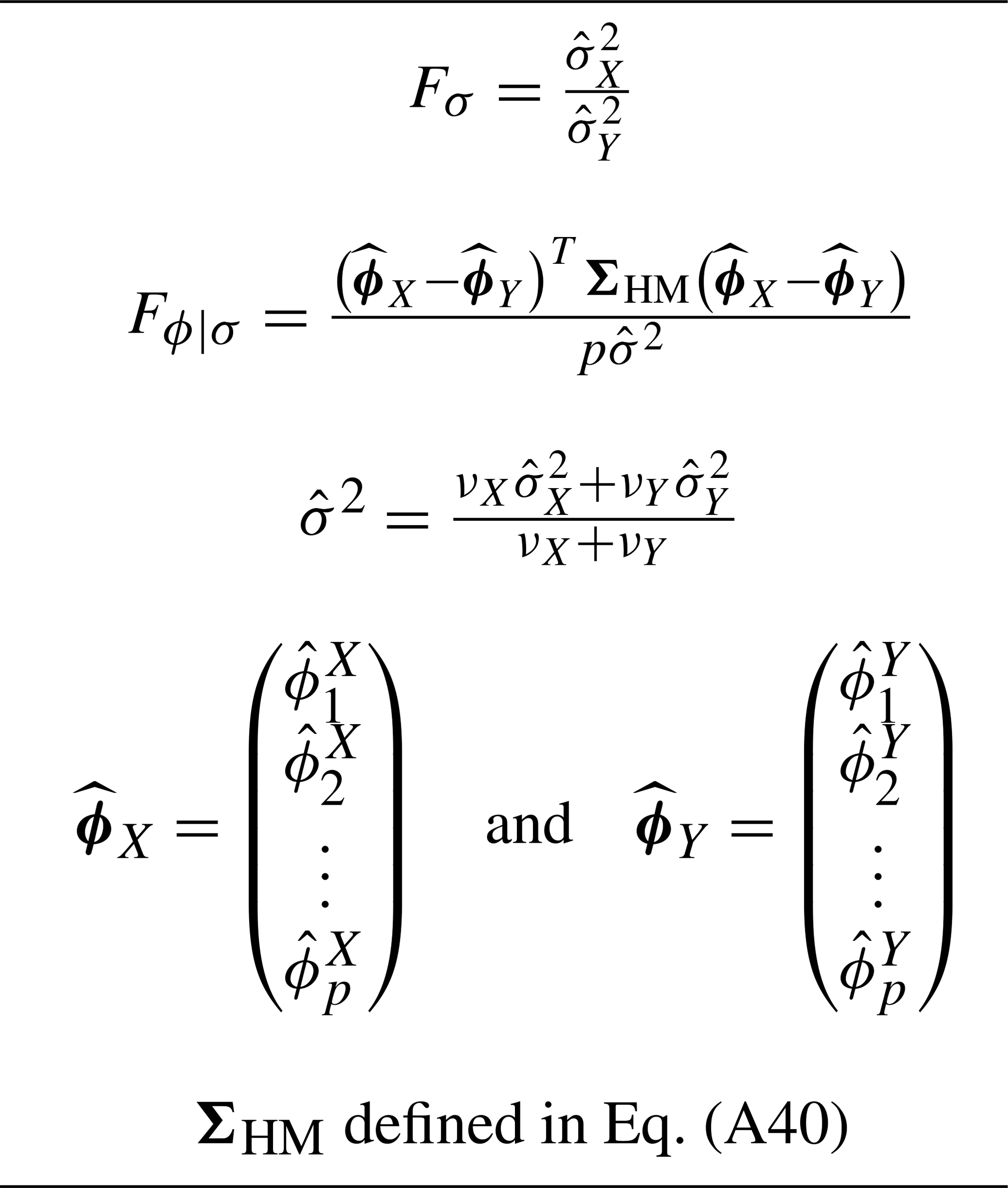
where . Then, the test of H0 is based on the statistic
where
and the remaining variables are defined in Table 1. Under the null hypothesis H0, it is shown in the Appendix that Fσ and Fϕ∣σ have the following approximate distributions:
Furthermore, the two statistics are independent. Critical values for Dσ and Dϕ∣σ are obtained individually from the critical values of the F-distribution, taking care to use the correct one-tailed or two-tailed test (see Appendix, particularly Eq. A31). In principle, the exact sampling distribution of Dϕ,σ can be derived analytically because Dϕ,σ is the sum of two random variables with known distributions. However, this analytic calculation is cumbersome, whereas the quantiles of can be estimated accurately and quickly by Monte Carlo techniques. Essentially, one draws random samples from and , substitutes these into Eqs. (18)–(19), evaluates Dϕ,σ in Eq. (17), and then repeats this many times (e.g., 10 000 times). Note that the required repetitions do not grow with sample size NX and NY since the F-distributions can be sampled directly. The 5 % significance threshold for Dϕ,σ, denoted Dcrit, is then obtained from the 95th percentile of the Monte Carlo samples. Although a Monte Carlo technique is used to obtain critical values, the test still constitutes a test for small sample sizes.
The above test assumes that time series come from an AR(p) process of known order and are excited by Gaussian noise. Grant and Quinn (2017) use Monte Carlo simulations to show that the test is robust to non-Gaussianity. Since our proposed method assumes normal distributions through Eqs. (20) and (21), its robustness to departures to Gaussian remains an open question and is a topic for future study. If the order of the process is unknown and has to be selected or the time series does not come from an autoregressive model (e.g., the process is a moving average process), then the type I error rate does not match its nominal value. In such cases, Grant and Quinn (2017) propose using some sufficiently large value of p, such as
where ⌊k⌋ denotes the largest integer smaller than or equal to k. The resulting AR(p*) model can capture the first auto-covariances regardless of their true origin. Of course, there will be some loss of power when a test based on p* is applied to a time series that comes from an AR(p) model with . This criterion seems to work well in our examples, as discussed in more detail in Sect. 5.
If a difference in the AR process is detected, then we would like to interpret those differences. After all, such comparisons often are motivated to validate climate models, so if a discrepancy is found we would like to describe those differences in meaningful terms. The fact that the statistic Dϕ,σ can be expressed as the sum of two independent terms suggests that it is natural to consider the two terms separately. The first term Dσ depends only on the difference in noise variance estimates and . The noise variance is the one-step prediction error of the AR model. After all, if the AR parameters in Eq. (11) were known exactly, then the conditional mean would be
where “S” stands for “signal”, and the one-step prediction error would be
Comparing the variance of one-step prediction errors is more statistically straightforward than comparing variances of the original time series because prediction errors are approximately uncorrelated, since they are the residuals of the AR model, which acts as a pre-whitening transformation. In contrast, comparing variances of time series is not straightforward because of serial correlation. In practice, the residuals are only approximately uncorrelated because the parameter values are only approximate.
The second term Dϕ∣σ vanishes when and is positive otherwise, hence it clearly measures the difference in AR parameters. To further interpret this term, it is helpful to partition the AR model for Xt into two parts, an unpredictable part associated with the noise and a predictable part SX. The predictable part is the response to the “initial condition”
With this notation, is the estimated predictable response of Xt. The estimated predictable response of Yt can be defined analogously and denoted . The initial conditions u may be drawn from the stationary distribution of Xt, the stationary distribution Yt, or some mixture of the two. In fact, the covariance matrix ΣHM defined in Eq. (A40) is proportional to the “harmonic mean” of the sample time-lagged covariance matrices for Xt and Yt. Assuming that the initial condition u is drawn from a distribution with covariance matrix ΣHM independently of u, then
If the initial condition for Xt and Yt is contrived to be the same u, then
Comparing this expression to Fϕ∣σ in Table 1 suggests that Fϕ∣σ is a kind of signal-to-noise ratio, where the “signal” is a difference in predictable responses for the same initial condition.
This difference in predictable responses, and hence Fϕ∣σ, can be related to the difference in R-squares of the individual time series. To see this, expand Eq. (27) as
The Cauchy–Schwarz inequality implies that
Hence, the above two expressions imply that
In the special case of equal noise variances, the above inequality becomes
where SNRX and SNRY are the signal-to-noise ratios of the two AR models:
Note that pFϕ∣σ is an estimate of the left-hand side of Eq. (31). Recall that R-square is defined as one minus the ratio of the noise variance to the total variance:
Because R-square and signal-to-noise ratio are one-to-one, inequality Eq. (31) implies the following: if the noise variances are identical, then a large difference in predictabilities (i.e., R-squares) necessarily implies a tendency for Fϕ∣σ to be large. This suggests that it may be informative to compare R-squares. We use the sample estimate
which is always between 0 and 1.
It should be recognized that a difference in R-square is a sufficient, but not necessary, condition for a difference in predictable responses. This fact can be seen from the fact that R-square for an AR(p) model is
In particular, two processes may have the same R-square because the combination of ϕs yields the same R-square, but the specific values of the ϕs may differ. Although a difference in R-squares is not a perfect indicator of Fϕ∣σ, it is at least a sufficient condition and therefore worth examination.
On the other hand, if the R-squares are the same, a difference in process still could be detected and should be explained. Simply identifying differences in ϕs would be unsatisfying because those differences have a complicated relation to the statistical characteristics of the process when p>1. Accordingly, we propose the following approach, which despite its limitations may still be insightful. Our basic idea is to choose initial conditions that maximize the mean square difference in predictable responses. To be most useful, we want this choice of initial condition to account for a multi-model comparison over M models. Accordingly, we define the mean square difference between predictable responses as
where
Our goal is to choose the initial condition u that maximizes Γ[u]. The initial condition u must be constrained in some way, otherwise Γ[u] is unbounded and there is no maximum. If the initial conditions are drawn from a distribution with covariance matrix ΣM, then an appropriate constraint is to fix the associated Mahalanobis distance:
The problem is now to maximize uTAu subject to the constraint . This is a standard optimization problem that is merely a generalization of principal component analysis (also called empirical orthogonal function analysis). The solution is obtained by solving the generalized eigenvalue problem
This eigenvalue problem yields p eigenvalues and p eigenvectors. The eigenvalues can be ordered from largest to smallest, , and the corresponding eigenvalues can be denoted . The first eigenvector u1 gives the initial condition that maximizes the sum square difference in predictable responses; the second eigenvector u2 gives the initial condition that maximizes Γ subject to the condition that ; and so on. The eigenvalues give the corresponding values of Γ. The eigenvectors can be collected into the p×p matrix
Because the matrices A and ΣM are symmetric, the eigenvectors can be chosen to satisfy the orthogonality property
Summing Γ over all eigenvectors gives
Note the similarity of the final expression to Eq. (27). This similarity implies that if only two models are compared and ΣM=ΣHM, then the solution exactly matches the variance of signal differences (27). Unfortunately, ΣHM and the noise variance depend on , so it is difficult to generalize the optimal initial condition to explain all pair-wise values of Fϕ∣σ. We suggest using a covariance matrix that is the harmonic mean across all M time series:
where is the sample covariance matrix of the initial condition Eq. (25) for the mth time series. Finally, we note that
Thus, λk∕Γsum is the fraction of sum total variance of signal differences explained by the kth eigenvector. Conceptually, each eigenvector uk can be interpreted as an initial condition that has been optimized to separate predictable responses.
To illustrate the proposed method, we apply it to an index of the Atlantic Meridional Overturning Circulation (AMOC). This variable is chosen because it is considered to be a major source of decadal variability and predictability (Buckley and Marshall, 2016; Zhang et al., 2019). However, the AMOC is not observed directly with sufficient frequency and consistency to constrain its variability on decadal timescales. As a result, there has been a heavy reliance on coupled atmosphere–ocean models to characterize AMOC variability and predictability. The question arises as to whether simulations of the AMOC by different models can be distinguished and, if so, how they differ.

Figure 1AMOC index simulated by 10 CMIP5 models under pre-industrial conditions. Each time series is offset by a constant with no re-scaling. The AMOC index is defined as the maximum annual mean meridional overturning streamfunction at 40∘ N in the Atlantic.
The data used in this study come from pre-industrial control runs from Phase 5 of the Coupled Model Intercomparison Project (CMIP5; Taylor et al., 2010). These control simulations lack year-to-year changes in forcing and thereby permit a focus on internal variability without confounding effects due to anthropogenic climate change. We consider only models that have pre-industrial control simulations spanning at least 500 years and contain meridional overturning circulation as an output variable. Only 10 models meet these criteria. An AMOC index is defined as the annual mean of the maximum meridional overturning streamfunction at 40∘ N in the Atlantic. A third-order polynomial over the 500 years is removed to eliminate climate drift. The AMOC index from the 10 models is shown in Fig. 1. Based on visual comparisons, one might perceive differences in amplitude (e.g., the MPI models tend to have larger amplitudes than other models) and differences in the degree of persistence (e.g., high-frequency variability is more evident in INMCM4 than in other models), but whether these differences are statistically significant remains to be established.
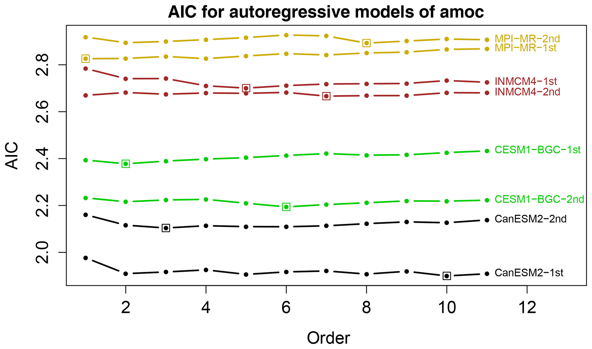
Figure 2Akaike's information criterion (AIC) as a function of autoregressive model order for AMOC time series from selected CMIP5 models. AIC is computed separately from the first and second 250 years of the data. A box identifies the minimum AIC up to order 11. The actual AIC values are shown – AIC values have not been offset. Models have been selected primarily to avoid line crossings.
To compare autoregressive processes, it is necessary to select the order of the autoregressive model. As discussed in Sect. 3, we use Eq. (22), which for ν=1.0 gives . One check on this choice is whether the residuals are white noise. We find that AR(5) is adequate for all models except MRI, in the sense that the residuals reveal no serious departures from white noise according to visual inspection and by the Ljung–Box test (Ljung and Box, 1978). Another check is to compute Akaike's information criterion (AIC; Box et al., 2008) for the two halves of the data (i.e., 250 years). Some representative examples are shown in Fig. 2. As can be seen, AIC is a relatively flat function of model order, hence small sampling variations can lead to large changes in order selection. Indeed, the order selected by AIC is sensitive to which half of the data is used. Nevertheless, because AIC is nearly a flat function of order, virtually any choice of order beyond AR(2) can be defended. The highest order selected by AIC is p=11. While we have performed our test for AR(11), this order would be a misleading illustration of the method because one might assume that 11 lags are necessary to identify model differences. Thus, in the results that follow, we choose AR(5) for all cases and bear in mind that comparisons with MRI may be affected by model inadequacy.
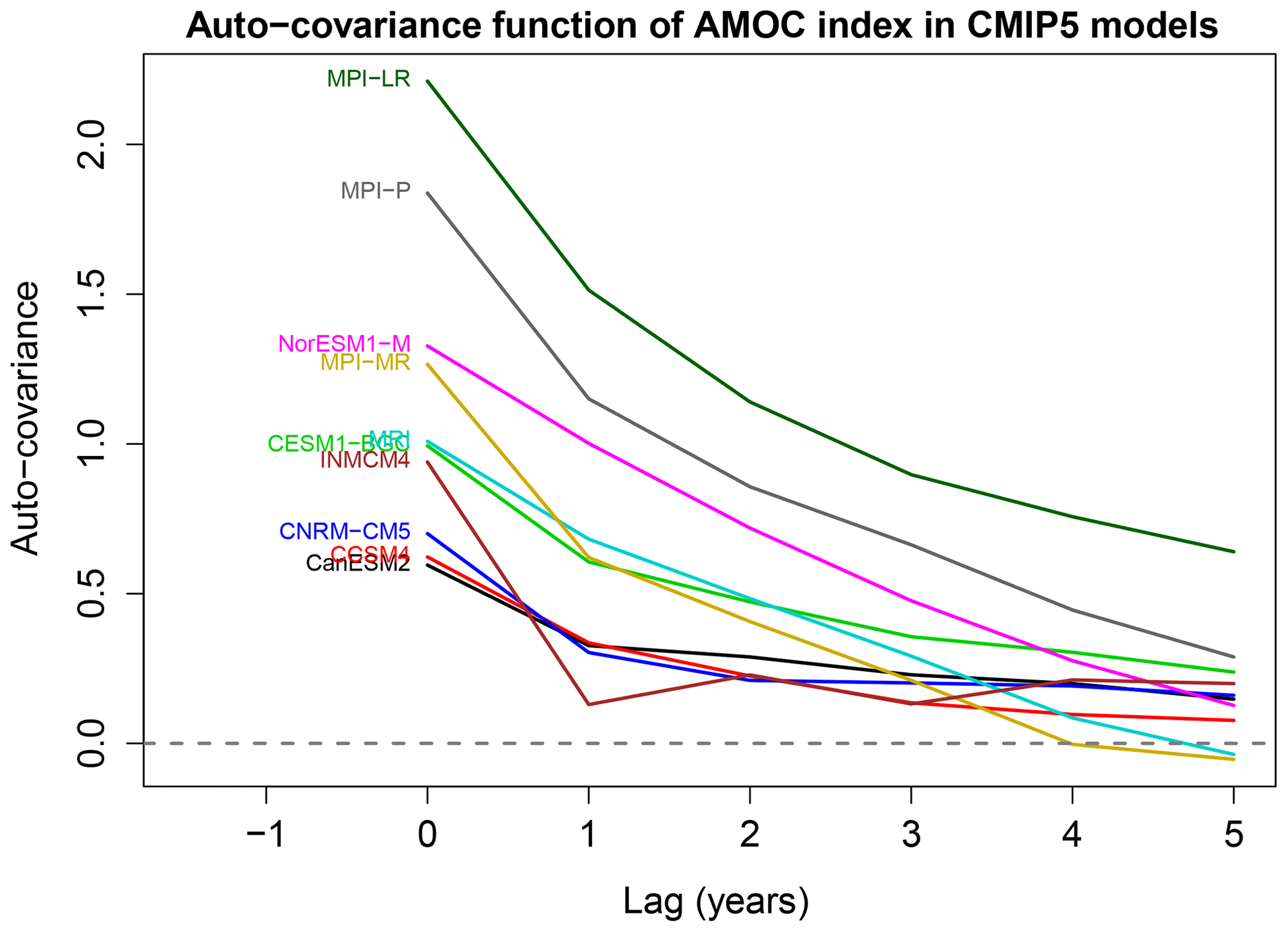
Figure 3Auto-covariance function of the AMOC time series from each CMIP5 model, as estimated from Eq. (6) using the first 250 years of data.
The choice of AR(5) means that all information relevant to deciding differences in stationary processes is contained in the first six values of the sample auto-covariance function . The sample auto-covariance function for each AMOC index is shown in Fig. 3. Recall that the zero-lag auto-covariance is the sample variance. The figure suggests that the time series have different variances and different decay rates, but it is unclear whether these differences are significant. Note that a standard difference-in-variance test cannot be performed here because the time series are serially correlated. One might try to modify the standard F-test by adjusting the degrees of freedom, as is sometimes advocated in the t-test (Zwiers and von Storch, 1995), but the adjustment depends on the autocorrelation function that we are trying to compare. An alternative approach is to pre-whiten the data based on the AR fit and then test differences in variance, but this is exactly equivalent to our test based on Fσ.
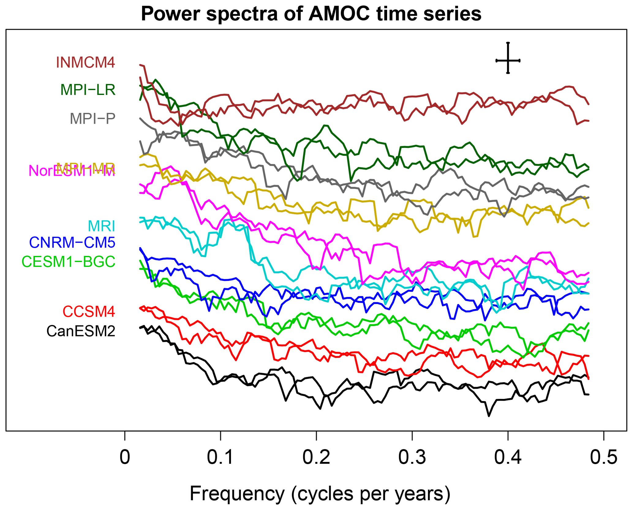
Figure 4Power spectra of AMOC time series from CMIP5 models. Spectra are estimated from the first and second 250 years of each time series using Daniell's estimator. The 95 % confidence interval and bandwidth are indicated by the error bars in the top right corner. The power spectra have been offset by a multiplicative constant to reduce overlap (the y axis is log scale). The longest resolved period is 60 years.
An alternative approach to comparing stationary processes is to compare power spectra. Power spectra of the AMOC time series are shown in Fig. 4. The spectra have been offset by a multiplicative constant to reduce overlap (otherwise the different curves would obscure each other). While many differences can be seen, the question is whether those differences are significant after accounting for sampling uncertainties. The two spectral tests discussed in Sect. 2 find relatively few differences between CMIP5 models, although they do indicate that time series from INMCM4 and MPI differ from those of other CMIP5 models (not shown). Presumably, these differences arise from the fact that the INMCM4 time series is closer to white noise and that the MPI time series have larger total variance than those from other CMIP5 models.
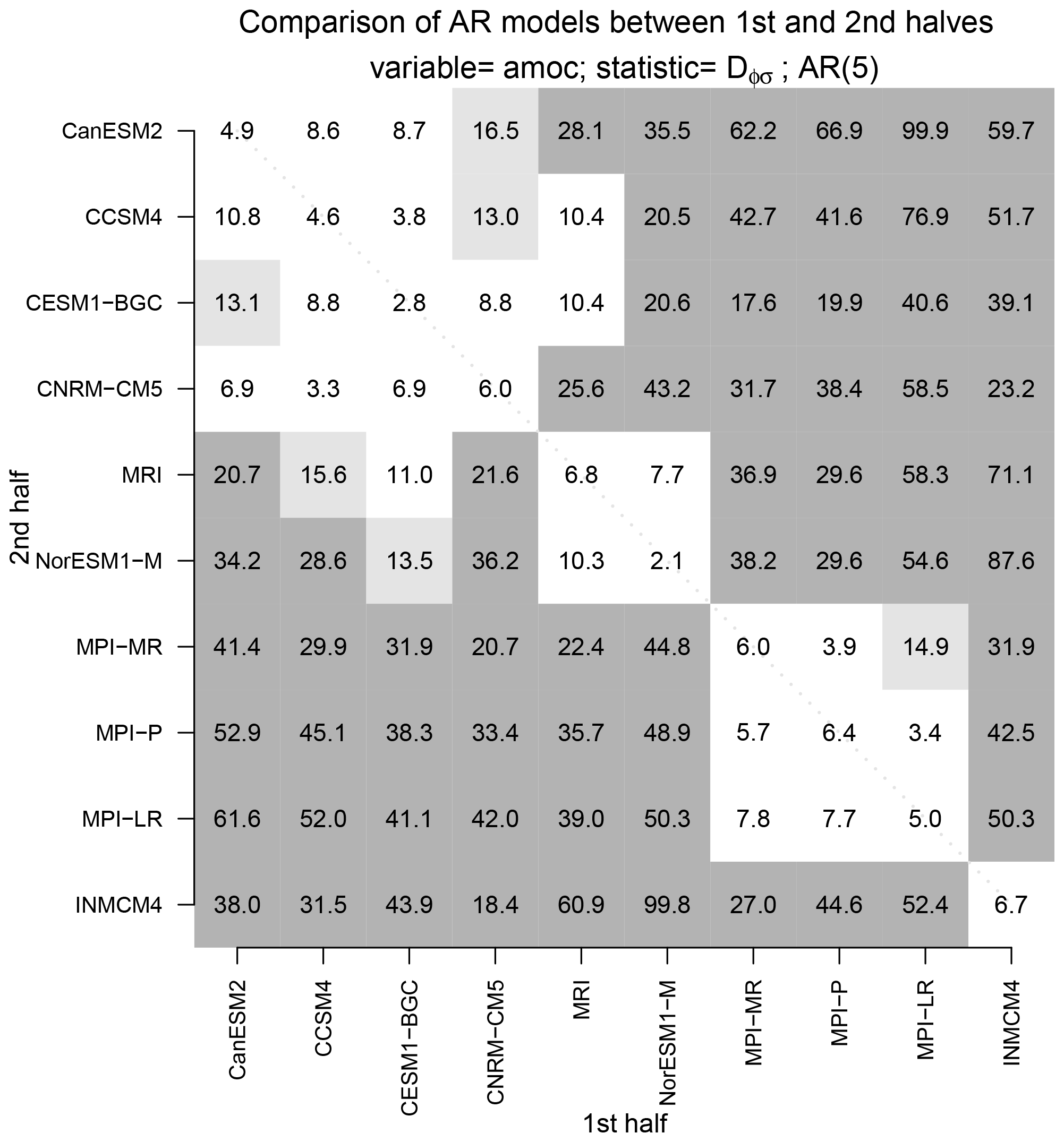
Figure 5A measure of the “distance” between AMOC time series between the first and second halves of CMIP5 pre-industrial control simulations. The distance is measured by the bias-corrected deviance statistic Dϕ,σ using an fifth-order AR model. The light and dark gray shadings show values exceeding the 5 % and 1 % significance levels, respectively (the threshold values are 12.7 and 17.0, respectively).
To illustrate our proposed method, we perform the following analysis. First, the AMOC index from each CMIP5 model is split into equal halves, each 250 years long. Then, each time series from the first half is compared to each time series in the second half. Some of these comparisons will involve time series from the same CMIP5 model. Our expectation is that no difference should be detected when time series from two different halves of the same CMIP5 model are compared. To summarize the comparisons, we show in Fig. 5 a matrix of the bias-corrected deviance statistic Dϕ,σ for every possible model comparison. This statistic is a measure of the “distance” between stationary process. The two shades of gray indicate a significant difference in AR process at the 5 % or 1 % level. Values along the diagonal correspond to comparisons of AMOC time series from the same CMIP5 model. No significant difference is detected when time series come from the same model. In contrast, significant differences are detected in most of the cases when the time series come from different CMIP5 models. Interestingly, models from the same institution tend to be indistinguishable from each other. For instance, the MPI models are mostly indistinguishable from each other, and the CCSM and CESM-BGC models (from the National Center for Atmospheric Research, NCAR) are mostly indistinguishable from each other. We say “mostly” because the difference depends on which half of the simulation is used in the comparison. For instance, a difference is detected when comparing the first half of the CESM1-BGC time series to the second half to the CCSM4 time series, but not vice versa. The models have been ordered to make natural clusters easy to identify in this figure. Aside from a few exceptions, the pattern of shading is the same for AR(2) and AR(10) models (not shown), demonstrating that our conclusion regarding significant differences in AR process is not sensitive to model order. Also, the pattern of shading is similar if the comparison is based on only from the first half of the simulations, or only from the second half of the simulations (not shown), indicating that our results are not sensitive to sampling errors.
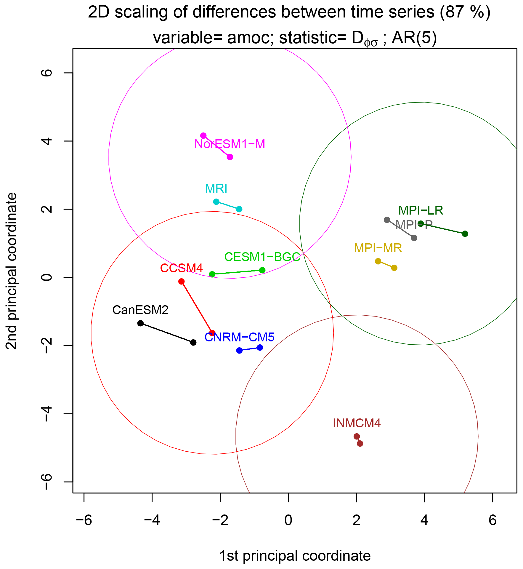
Figure 6A set of points in a two-dimensional Cartesian plane whose pair-wise Euclidean distances most closely approximate the pair-wise distances between autoregressive processes of AMOC time series. The difference between AR processes is measured by the bias-corrected deviance statistic Dϕ,σ and the points are identified using multidimensional scaling techniques. There are 20 points corresponding to 10 CMIP5 models, each model time series being split in half. Time series from the same model have the same color and are joined by a line segment. Circles around selected points enclose models whose time series are statistically indistinguishable from that of the center model at the 5 % significance level.
To visualize natural clusters more readily, we identify a set of points in a cartesian plane whose pair-wise distances match the above distances as closely as possible. These points can be identified using a procedure called multidimensional scaling (Izenman, 2013). The procedure is to compute the deviance statistic between every possible pair of time series. Because there are 10 CMIP models and time series from each model is split in half, there are 20 time series being compared. Thus, the deviance statistic for every possible pair can be summarized in a 20×20 distance matrix. From this matrix, multidimensional scaling can find the set of points in a 20-dimensional space that has this distance matrix. Moreover, it can find the points in a two-dimensional space whose distance matrix most closely approximates the original distance matrix in some objective sense. In our case, 87 % of original distance matrix can be represented by two-dimensional points. These points are shown in Fig. 6. Although 87 % of the distance matrix is represented in this figure, isolated points may have relatively large discrepancies. The average discrepancy is about 2 units, with the largest discrepancy being about 3.6 units between MRI and MPI-LR. An attractive feature of this representation is that the decision rule for statistical significance, , is approximately equivalent to drawing a circle of radius around a point and identifying all the points that lie outside that circle. This geometric procedure would be exact in a 20-dimensional space, but is only approximate in the 2-dimensional space shown in Fig. 6. The figure suggests that the MPI models and INMCM4 form their own natural clusters. For other models, a particular choice of clusters is shown in the figure, but this is merely an example, and different clusters with different groupings could be justified. Note that all line segments connecting results from the same CMIP model are shorter than the circle radius, indicating no significant difference between time series from the same CMIP model.
It is interesting to relate the above differences to the auto-covariance functions shown in Fig. 3. It is likely that INMCM4 differs from other models because its auto-covariance function decays most quickly to zero. The MPI models are distinguished from the others by their large variances. Interestingly, note that the auto-covariance function for NorESM1-M is intermediate between that of two MPI models, yet the test indicates that NorESM1-M differs from the MPI models. Presumably, the MPI models are indistinguishable because their auto-covariance functions have the same shape, including a kink at lag 1, whereas the NorESM1-M model has no kink at lag 1. This example illustrates that the test does not behave like a mean square difference between auto-covariance functions, which would cluster NorESM1-M with the MPI models.
It is worth clarifying how the above clustering technique differs from those in previous studies. Piccolo (1990) proposed a distance measure based on the Euclidean norm of the difference in AR parameters, namely
In contrast, our hypothesis test uses a Mahalanobis norm for measuring differences in AR parameters, where the covariance matrix is based on the sample covariance matrices of the time-lagged data (see Eq. A44). While the Euclidean norm Eq. (45) does have some attractive properties as discussed in Piccolo (1990), it is inconsistent with the corresponding hypothesis test for differences in AR parameters. As a result, the resulting cluster may emphasize differences with large Euclidean norms that are insignificant, or may downplay differences in small Euclidean norms that are significant. In contrast, the distance measure used in our study is consistent with a rigorous hypothesis test. Maharaj (2000) proposes a classification procedure that is consistent with hypothesis testing, but that hypothesis test does not account for differences in noise variances.
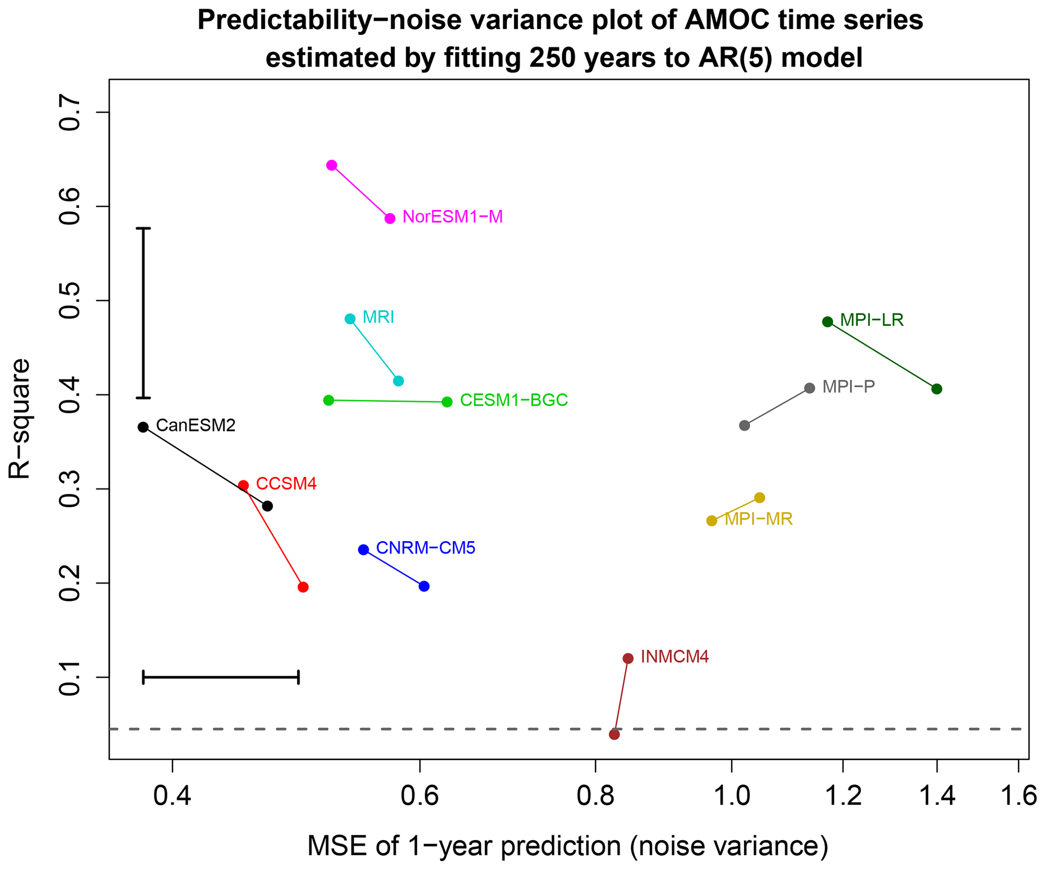
Figure 7Noise variance versus the R-square of AR(5) models estimated from 250-year segments of AMOC time series from 10 CMIP5 models. Estimates from the same CMIP5 model have the same color and are joined by a line segment. The error bar in the bottom left corner shows the critical distance for a significant difference in noise variance at the 5 % level. The x axis is on a log scale so that equal variance ratios correspond to equal linear distances. The error bar in the upper left shows a 95 % confidence interval for R-square using the method of Lee (1971) and computed from the MBESS package in R. The dashed line is the 5 % significance threshold for the R-square.
Having identified differences between stationary processes, it is of interest to relate those differences to standard properties of the time series. Recall that our measure of the difference between stationary processes Dϕ,σ is the sum of two other measures, namely Dσ and Dϕ∣σ. Measure Dσ depends only on the noise variances, that is, it depends on the mean square error of a 1-year prediction. In contrast, Dϕ∣σ measures the difference in predictable responses of the process. As discussed in Sect. 4, we suggest examining differences in R-square. A graph of the noise variance plotted against R-square of each autoregressive model is shown in Fig. 7. The error bars show the critical distance for a significance difference in noise variance (lower left) and for a difference in R-square (upper right). First note that the projections of line segments onto the x axis or y axis are shorter than the respective error bars, indicating that differences in noise and differences in predictability are insignificant when estimated from the same CMIP5 model. Second, note that the relative positions of the dots are similar to those in Fig. 6. Thus, the noise variance and R-square appear to be approximate “principal coordinates” for distinguishing univariate autoregressive processes. Third, using noise variances alone, the MPI models would be grouped together, then INMCM4 would be grouped by itself, while at the bottom end CanESM2 and CCSM4 would be grouped together. These groupings are consistent with the clusters identified above using the full distance measure Dϕ,σ, suggesting that differences in noise variances explain the major differences between stationary processes. Fourth, the AR models have R-square values mostly between 0.25 and 0.5. Time series from INMCM4 have the smallest R-square values while time series from NorESM1 have the largest R-square values.
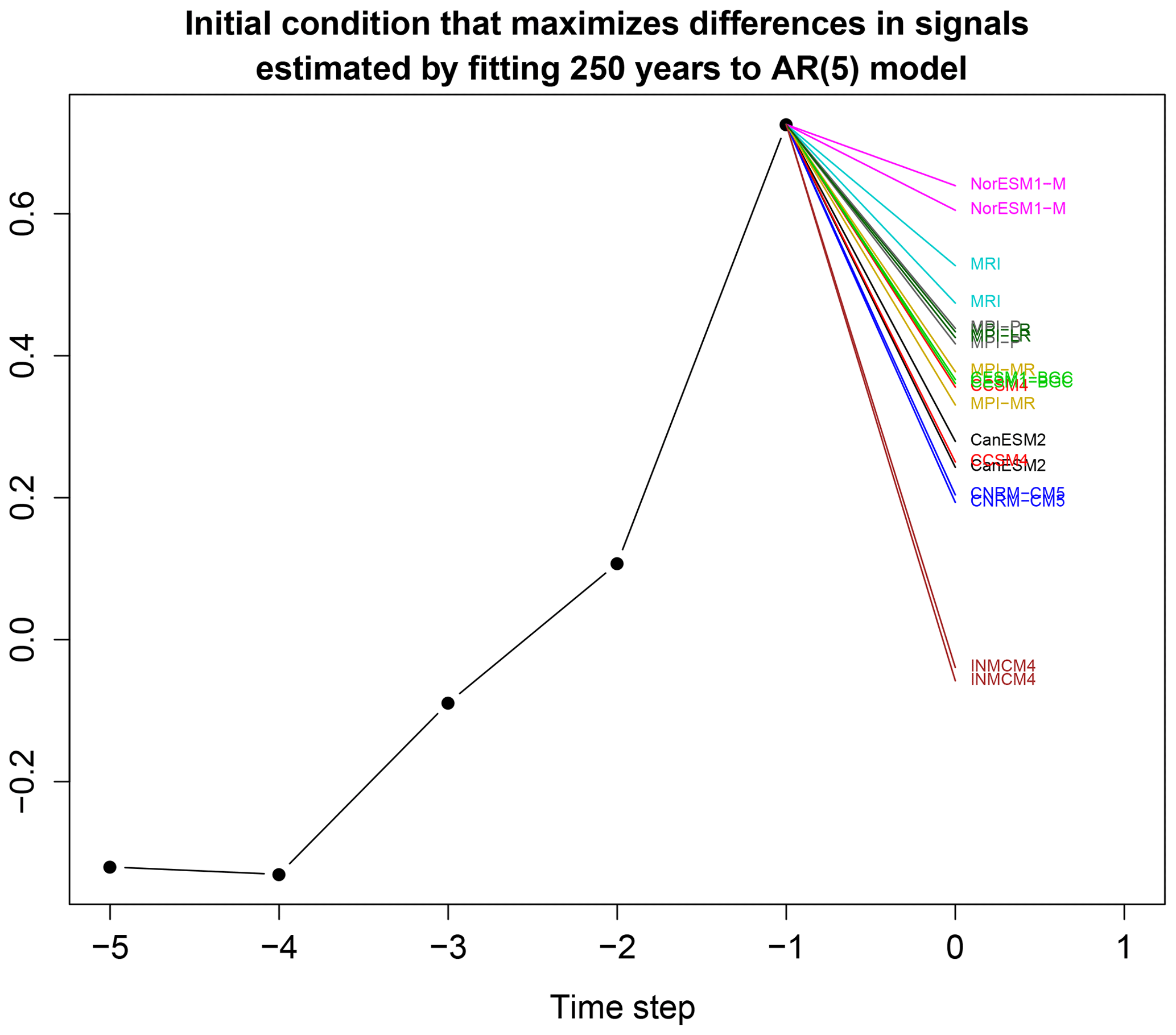
Figure 8Predictions from each estimated AR(5) model using the optimal initial condition derived from Eq. (39). The optimal initial condition is the five black dots joined by lines, and the resulting predictions are the colored lines. Each CMIP model has two predictions corresponding to the two AR(5) models estimated from two non-overlapping 250-year time series from the same CMIP model.
An alternative approach to describing differences in AR parameters is to show differences in response to the same initial condition. We use the optimization method discussed in Sect. 4 to find the initial condition that maximizes the sum square difference in responses. The result is shown in Fig. 8. Essentially, the models separate by predictability – the order of the models from top to bottom closely tracks the order of the models based on R-square seen in Fig. 7. For this initial condition, INMCM4 damps nearly to zero in one time step, whereas NorESM1-M decays the slowest among the models, consistent with expectations from R-square. This initial condition explains 82 % of the differences in response. Because optimal initial conditions form a complete set, an arbitrary initial condition can be represented as a linear combination of optimal initial conditions. If the AR models were used to predict an observational time series with covariance matrix ΣM, then most differences between model predictions could be explained by the differences in response to a single optimal initial condition.
We end with a brief summary of our exploration of the χ2 statistic proposed by Lund et al. (2009). As mentioned earlier, the result is sensitive to the choice of K. However, instead of summing based on the cutoff parameter K, we summed over all possible lags, and set all sample auto-covariances beyond lag p to zero. Using this approach, we find that the resulting χ2 statistic gives results very similar to ours for p=5, including clustering the MPI models with each other, and separating them from NorEMS1-M. We have not investigated this procedure sufficiently to propose it as a general rule but mention it to suggest the possibility that some alternative rule for computing the sum Eq. (9) may yield reasonable results.
This paper examined tests for differences in stationary processes and proposed a new approach to characterizing those differences. The basic idea is to fit each time series to an autoregressive model and then test for differences in parameters. The likelihood ratio test for this comparison was derived in Maharaj (2000) and Grant and Quinn (2017). We have modified the test to correct for certain biases and to include a test for differences in noise variance. The latter test is of major interest in climate applications and leads to considerable simplifications in estimation and interpretation. Furthermore, the proposed test is applicable to small samples. In addition, we propose new approaches to interpreting and visualizing differences in stationary processes. The procedure was illustrated on AMOC time series from pre-industrial control simulations of 10 models in the CMIP5 archive. Based on time series 250 years in length, the procedure was able to distinguish about four clusters of models, where time series from the same CMIP5 model are grouped together in the same cluster. These clusters are identified easily using a multidimensional technique. The clusters obtained by this method were not sensitive to the order of the autoregressive model, although the number of significant differences decreases with AR order due to the larger number of parameters being estimated. Further analysis shows that these clusters can be explained largely by differences in 1-year prediction errors in the AR models and differences in R-square.
The proposed method can be used to compare any stationary time series that are well fit by an autoregressive model, which includes most climate time series. Thus, this method could be used to decide whether two climate models generate the same temporal variability. A natural question is whether this approach can be generalized to compare multivariate time series. This generalization will be developed in Part 2 of this paper. The method also could be used to compare model simulations to observations, provided that the stationarity assumption is satisfied. If non-stationarity is strong, then this method would need to be modified to account for such non-stationarity, such as adding exogenous terms to the AR model. The likelihood-ratio framework can accommodate such extensions and will be developed in Part 3 of this paper.
In this Appendix, we derive a test for equality of parameters of autoregressive models based on the likelihood ratio test. The derivation is similar to that in Maharaj (2000) and Grant and Quinn (2017), except modified to test for differences in noise variance and to correct for known biases in maximum likelihood estimates. In addition, we show how the bias-corrected likelihood ratio can be partitioned into two independent ratios and derive the sampling distributions for each.
We consider only the conditional likelihood, which is the likelihood function conditioned on the first p values of the process. The conditional likelihood approach is reasonable for large sample sizes and has the advantage that the estimates can be obtained straightforwardly from the method of least squares. Suppose we have a time series of length NX for Xt. Then the conditional likelihood function for Xt is
(see Eq. A7.4.2b of Box et al., 2008). The maximum likelihood estimates of the parameters, denoted by , are obtained from the method of least squares. The maximum likelihood estimate of is
Substituting this into the likelihood function Eq. (A1) and then taking −2 times the logarithm of the likelihood function gives
Similarly, suppose we have a time series of length NY for Yt. Then, the corresponding likelihood function is
the maximum likelihood estimate of is
and −2 times the logarithm of the likelihood function is
Because Xt and Yt are independent, the likelihood function for all the data is the product LXLY.
Under hypothesis H0, the likelihood function has the same form as LXLY, except there is only a single set of autoregressive parameters and a single noise variance σ. The corresponding likelihood function is therefore
The maximum likelihood estimates of , denoted , are obtained from the least squares estimates of the pooled sample. Again, these estimates are obtained easily by the method of least squares. The maximum likelihood estimate of the common variance σ2 is
The corresponding log-likelihood is
Finally, we compute the likelihood ratio, or equivalently, the difference in the log-likelihood functions. This difference (multiplied by −2) is called the deviance statistic and is
It is well known that maximum likelihood estimates of variance are biased. Accordingly, we define bias-corrected deviance statistics before proceeding. This can be done by replacing sample sizes by degrees of freedom. Care must be exercised in such substitutions because replacing MLEs with unbiased versions will yield likelihoods that are no longer maximized, and therefore may yield deviance statistics that are negative. Our goal is to define a bias-corrected deviance statistic that is non-negative
To compute the degrees of freedom, note that the sample size of Xt is NX−p, because the first p time steps are excluded from the conditional likelihood, and p+1 parameters are being estimated, so the degrees of freedom is the difference, . Similarly, the degrees of freedom for Yt is . Let the degrees of freedom be denoted
Accordingly, an unbiased estimate of is
and an unbiased estimate of is
As will be shown below, the appropriate bias correction for is
Also, it proves helpful to define the unbiased estimate of the common variance σ2 as
Then, the bias-corrected deviance statistic Eq. (A9) can be defined as
where
We now prove the Dσ and Dϕ∣σ are non-negative, independent, and have sampling distributions related to the F-distribution. To show that Dσ is non-negative, note that the ratio in Eq. (A16) is the weighted arithmetic mean over the weighted geometric mean of and . Consequently, we may invoke the AM-GM inequality to show that Dσ is non-negative and vanishes if and only if . In this sense, Dσ measures the “distance” between and . Incidentally, had we used the uncorrected likelihoods, the resulting deviance statistic would vanish at , which would give a biased measure of deviance.
To prove the remaining properties of Dσ and Dϕ∣σ, we adopt a vector notation that is better suited to the task. Accordingly, let the AR(p) model Eq. (11) be denoted
where wX is an (NX−p)-dimensional vector, ZX is a matrix, j is a (NX−p)-dimensional vector of ones, γx is a scalar, and the remaining terms have been defined previously.
Since H0 does not restrict γX, it proves convenient to eliminate this parameter by projecting onto the complement of j. Therefore, we multiply both sides of the equation by the projection matrix
This multiplication has the effect of eliminating the γX term and centering each column of wX and ZX. Henceforth, we assume that each column of wX and ZX has been centered. One should remember that the degrees of freedom associated with estimating the noise variance should be reduced by one to account for this pre-centering of the data. Similarly, the corresponding model for Yt in Eq. (12) is written as
where wY is an (NY−p)-dimensional vector, and the remaining terms are analogous to those in Eq. (A18). As for X, we assume that each column of wY and ZY is centered. The least squares estimates for ϕX and ϕY are
and the corresponding sum square errors are
where denotes the Euclidean norm of vector a. The sum square errors are related to the estimated variances as
Following the standard theory of least squares estimation for the general linear model, Brockwell and Davis (1991; Sect. 8.9) suggest that the sum square errors have the following approximate chi-squared distributions:
Because Xt and Yt are independent, the associated sum square errors are independent, hence under H0, the statistic
has an F-distribution with (νX,νY) degrees of freedom, as stated in Eq. (20). Furthermore, if H0 is true, then
has a (scaled) chi-squared distribution with νX+νY degrees of freedom; i.e.,
Straightforward algebra shows that Dϕ in Eq. (A16) can be written as a function of Fσ as
This is a U-shaped function with a minimum value of zero at Fσ=1 and monotonic on either side of Fσ=1. Note that if Xt and Yt were swapped, then the X and Y labels would be swapped and , which yields the same value of Dσ. Let denote the critical value such that has probability α when F has an F-distribution with (νX,νY) degrees of freedom. Then, the α100 % significance threshold for rejecting H0 is
where α on the right-hand side is divided by 2.
The least squares estimate of the common regression parameters ϕ is
and the corresponding sum square error is
We now express this in terms of parameter estimates of the individual AR models. To do this, we invoke the standard orthogonality relation
It follows that
The difference between least squares estimates and is
while that between and is
Substituting these expressions into Eq. (A36) and invoking Eq. (A28) yields
where
ΣHM is proportional to the harmonic mean of two covariance matrices. This matrix arises naturally if we recall the fact that the sample estimates of the parameters have the following distributions:
Therefore, under H0,
hence
Again, by analogy with the standard theory of least squares estimation for the general linear model, SSEσ and the quadratic form in Eq. (A39) are approximately independent of each other. Thus, if H0 is true, then
has an approximate F-distribution with degrees of freedom, as indicated in Eq. (21). Using the identity
it follows that
and therefore
It is clear that Fϕ∣σ is non-negative, and therefore Dϕ∣σ is non-negative. Furthermore, Dϕ∣σ is a monotonic function of Fϕ|σ. Therefore, the α100 % significance threshold for rejecting H0 is
It remains to define the critical value for rejecting H0 based on Dϕ,σ. Dσ and Dϕ∣σ are independent because Dσ depends on the ratio of and , while Dϕ∣σ depends on the sum , and the ratio and sum are independent as a consequence of Lukacs' proportion-sum independence theorem (Lukacs, 1955). Therefore, we may sample from the F-distributions (20) and (21) and then use Monte Carlo techniques to estimate the upper α100th percentile of under H0.
An R function for performing the test proposed in this paper is available from the authors upon request.
Both authors participated in the writing and editing of the manuscript. TD performed the numerical calculations.
The authors declare that they have no conflict of interest.
We thank Martha Buckley, Robert Lund, and two anonymous reviewers for comments that led to improvements in the presentation of this work. This research was supported primarily by the National Oceanic and Atmospheric Administration (NA16OAR4310175). The views expressed herein are those of the authors and do not necessarily reflect the views of these agencies.
This research has been supported by the NOAA (grant no. NA16OAR4310175).
This paper was edited by Seung-Ki Min and reviewed by two anonymous referees.
Box, G. E. P., Jenkins, G. M., and Reinsel, G. C.: Time Series Analysis: Forecasting and Control, Wiley-Interscience, 4th Edn., 2008. a, b, c, d
Brockwell, P. J. and Davis, R. A.: Time Series: Theory and Methods, Springer Verlag, 2nd Edn., 1991. a
Brockwell, P. J. and Davis, R. A.: Introduction to Time Series and Forecasting, Springer, 2002. a
Buckley, M. W. and Marshall, J.: Observations, inferences, and mechanisms of the Atlantic Meridional Overturning Circulation: A review, Rev. Geophys., 54, 5–63, https://doi.org/10.1002/2015RG000493, 2016. a
Coates, D. S. and Diggle, P. J.: Test for comparing two estimated spectral densities, J. Time Ser. Anal., 7, 7–20, 1986. a, b
Grant, A. J. and Quinn, B. G.: Parametric Spectral Discrimination, J. Time Ser. Anal., 38, 838–864, https://doi.org/10.1111/jtsa.12238, 2017. a, b, c, d, e, f, g, h, i
Izenman, A. J.: Modern Mutivariate Statistical Techniques: Regression, Classification, and Manifold Learning, Springer, corrected 2nd printing Edn., 2013. a
Jenkins, G. M. and Watts, D. G.: Spectral Analysis and its Applications, Holden-Day, 1968. a
Lee, Y.-S.: Some Results on the Sampling Distribution of the Multiple Correlation Coefficient, J. Roy. Stat. Soc. Ser. B, 33, 117–130, 1971. a
Ljung, G. M. and Box, G. E. P.: On a measure of lack of fit in time series models, Biometrika, 65, 297–303, 1978. a
Lukacs, E.: A Characterization of the Gamma Distribution, Ann. Math. Statist., 26, 319–324, https://doi.org/10.1214/aoms/1177728549, 1955. a
Lund, R., Bassily, H., and Vidakovic, B.: Testing Equality of Stationary Autocovariances, J. Time Ser. Anal., 30, 332–348, 2009. a, b, c, d, e, f, g, h, i
Maharaj, E. A.: Cluster of Time Series, J. Classification, 17, 297–314, https://doi.org/10.1007/s003570000023, 2000. a, b, c, d, e, f, g
Piccolo, D.: A Distance Measure for Classifying ARIMA Models, J. Time Ser. Anal., 11, 153–164, https://doi.org/10.1111/j.1467-9892.1990.tb00048.x, 1990. a, b, c
Taylor, K. E., Stouffer, R. J., and Meehl, G. A.: A summary of the CMIP5 experimental design, available at: https://pcmdi.llnl.gov/mips/cmip5/experiment_design.html (last access: 6 October 2020), 2010. a
Zhang, R., Sutton, R., Danabasoglu, G., Kwon, Y.-O., Marsh, R., Yeager, S. G., Amrhein, D. E., and Little, C. M.: A Review of the Role of the Atlantic Meridional Overturning Circulation in Atlantic Multidecadal Variability and Associated Climate Impacts, Rev. Geophys., 57, 316–375, https://doi.org/10.1029/2019RG000644, 2019. a
Zwiers, F. W. and von Storch, H.: Taking Serial Correlation into Account in Tests of the Mean, J. Climate, 8, 336–351, 1995. a
- Abstract
- Introduction
- Previous methods for comparing time series
- Comparing autoregressive models
- Interpretation of differences in AR processes
- Example: diagnosing differences in AMOC simulations
- Conclusions
- Appendix A: Derivation of the test
- Code availability
- Author contributions
- Competing interests
- Acknowledgements
- Financial support
- Review statement
- References
- Article
(3508 KB) - Full-text XML
- Abstract
- Introduction
- Previous methods for comparing time series
- Comparing autoregressive models
- Interpretation of differences in AR processes
- Example: diagnosing differences in AMOC simulations
- Conclusions
- Appendix A: Derivation of the test
- Code availability
- Author contributions
- Competing interests
- Acknowledgements
- Financial support
- Review statement
- References